Biomedical image segmentation is a vital task in the analysis of medical imaging, including the detection and delineation of pathological regions or anatomical structures within medical images. It has played a pivotal role in a variety of medical applications, involving diagnoses, monitoring of diseases, and treatment planning. Conventionally, clinicians or expert radiologists have manually conducted biomedical image segmentation, which is prone to human error, subjective, and time-consuming. With the advancement in computer vision and deep learning (DL) algorithms, automated and semi-automated segmentation techniques have attracted much research interest. DL approaches, particularly convolutional neural networks (CNN), have revolutionized biomedical image segmentation. With this motivation, we developed a novel equilibrium optimization algorithm with a deep learning-based biomedical image segmentation (EOADL-BIS) technique. The purpose of the EOADL-BIS technique is to integrate EOA with the Faster RCNN model for an accurate and efficient biomedical image segmentation process. To accomplish this, the EOADL-BIS technique involves Faster R-CNN architecture with ResNeXt as a backbone network for image segmentation. The region proposal network (RPN) proficiently creates a collection of a set of region proposals, which are then fed into the ResNeXt for classification and precise localization. During the training process of the Faster RCNN algorithm, the EOA was utilized to optimize the hyperparameter of the ResNeXt model which increased the segmentation results and reduced the loss function. The experimental outcome of the EOADL-BIS algorithm was tested on distinct benchmark medical image databases. The experimental results stated the greater efficiency of the EOADL-BIS algorithm compared to other DL-based segmentation approaches.
Citation: Eman A. Al-Shahari, Marwa Obayya, Faiz Abdullah Alotaibi, Safa Alsafari, Ahmed S. Salama, Mohammed Assiri. Accelerating biomedical image segmentation using equilibrium optimization with a deep learning approach[J]. AIMS Mathematics, 2024, 9(3): 5905-5924. doi: 10.3934/math.2024288
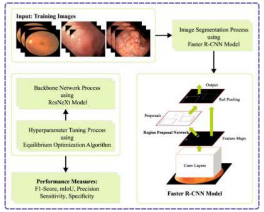
Biomedical image segmentation is a vital task in the analysis of medical imaging, including the detection and delineation of pathological regions or anatomical structures within medical images. It has played a pivotal role in a variety of medical applications, involving diagnoses, monitoring of diseases, and treatment planning. Conventionally, clinicians or expert radiologists have manually conducted biomedical image segmentation, which is prone to human error, subjective, and time-consuming. With the advancement in computer vision and deep learning (DL) algorithms, automated and semi-automated segmentation techniques have attracted much research interest. DL approaches, particularly convolutional neural networks (CNN), have revolutionized biomedical image segmentation. With this motivation, we developed a novel equilibrium optimization algorithm with a deep learning-based biomedical image segmentation (EOADL-BIS) technique. The purpose of the EOADL-BIS technique is to integrate EOA with the Faster RCNN model for an accurate and efficient biomedical image segmentation process. To accomplish this, the EOADL-BIS technique involves Faster R-CNN architecture with ResNeXt as a backbone network for image segmentation. The region proposal network (RPN) proficiently creates a collection of a set of region proposals, which are then fed into the ResNeXt for classification and precise localization. During the training process of the Faster RCNN algorithm, the EOA was utilized to optimize the hyperparameter of the ResNeXt model which increased the segmentation results and reduced the loss function. The experimental outcome of the EOADL-BIS algorithm was tested on distinct benchmark medical image databases. The experimental results stated the greater efficiency of the EOADL-BIS algorithm compared to other DL-based segmentation approaches.

| [1] |
S. Chakraborty, K. Mali, An overview of biomedical image analysis from the deep learning perspective, Research Anthology on Improving Medical Imaging Techniques for Analysis and Intervention, 2023, 43–59. https://doi.org/10.4018/978-1-6684-7544-7.ch003 doi: 10.4018/978-1-6684-7544-7.ch003

|
| [2] |
N. S. Punn, S. Agarwal, Modality specific U-Net variants for biomedical image segmentation: a survey, Artif. Intell. Rev., 55 (2022), 5845–5889. https://doi.org/10.4018/978-1-6684-7544-7.ch003 doi: 10.4018/978-1-6684-7544-7.ch003
|
| [3] |
M. Yeung, L. Rundo, Y. Nan, E. Sala, C.B. Schönlieb, G. Yang, Calibrating the Dice loss to handle neural network overconfidence for biomedical image segmentation, J. Digit. Imaging, 36 (2023), 739–752. https://doi.org/10.1007/s10278-022-00735-3 doi: 10.1007/s10278-022-00735-3
|
| [4] |
A. Lou, S. Guan, M. Loew, Cfpnet-m: A lightweight encoder-decoder-based network for multimodal biomedical image real-time segmentation, Comput. Biol. Med., 154 (2023), 106579. https://doi.org/10.1016/j.compbiomed.2023.106579 doi: 10.1016/j.compbiomed.2023.106579
|
| [5] | K. A. Davamani, C. R. Robin, S. Amudha, L. J. Anbarasi, Biomedical image segmentation by deep learning methods, Computational Analysis and Deep Learning for Medical Care: Principles, Methods, and Applications, 2021,131–154. https://doi.org/10.1002/9781119785750.ch6 |
| [6] | A. Shrivastava, M. Chakkaravathy, M. A. Shah, A Comprehensive Analysis of Machine Learning Techniques in Biomedical Image Processing Using Convolutional Neural Networks, In: 2022 5th International Conference on Contemporary Computing and Informatics (IC3I), 2022, 1363–1369. IEEE. https://doi.org/10.1109/IC3I56241.2022.10072911 |
| [7] | A. Iqbal, M. Sharif, M. A. Khan, W. Nisar, M. Alhaisoni, FF-UNet: A U-shaped deep convolutional neural network for multimodal biomedical image segmentation, Cogn. Comput., 14 (2022.), 1287–1302. https://doi.org/10.1007/s12559-022-10038-y |
| [8] | N. S. Punn, S. Agarwal, BT-Unet: A self-supervised learning framework for biomedical image segmentation using barlow twins with U-net models. Machine Learning, 111 (2022), 4585–4600. https://doi.org/10.1007/s10994-022-06219-3 |
| [9] | A. J. Larrazabal, C. Martínez, J. Dolz, E. Ferrante, Orthogonal ensemble networks for biomedical image segmentation, In: Medical Image Computing and Computer Assisted Intervention–MICCAI 2021: 24th International Conference, Strasbourg, France, September 27–October 1, 2021, Proceedings, Part Ⅲ 24,594–603. Springer International Publishing. https://doi.org/10.1007/978-3-030-87199-4_56 |
| [10] | Q. Liu, H. Jiang, T. Liu, Z. Liu, S. Li, W. Wen, Y. Shi, Defending deep learning-based biomedical image segmentation from adversarial attacks: A low-cost frequency refinement approach. In: Medical Image Computing and Computer Assisted Intervention–MICCAI 2020: 23rd International Conference, Lima, Peru, October 4–8, 2020, Proceedings, Part IV 23,342–351. Springer International Publishing. https://doi.org/10.1007/978-3-030-59719-1_34 |
| [11] | J. Zhang, Y. Zhang, Y. Jin, J. Xu, X. Xu, MDU-Net: multi-scale densely connected U-Net for biomedical image segmentation, Health Information Science and Systems, 11 (2023), 13. https://doi.org/10.1007/978-3-030-59719-1_34 |
| [12] |
S. Pan, X. Liu, N. Xie, Y. Chong, EG-TransUNet: A transformer-based U-Net with enhanced and guided models for biomedical image segmentation, BMC Bioinformatics, 24 (2023), 85. https://doi.org/10.1007/978-3-030-59719-1_34 doi: 10.1007/978-3-030-59719-1_34
|
| [13] | N. K. Tomar, D. Jha, M. A. Riegler, H. D. Johansen, D. Johansen, J. Rittscher, et al., Fanet: A feedback attention network for improved biomedical image segmentation, IEEE Transactions on Neural Networks and Learning Systems, 2022. https://doi.org/10.1109/TNNLS.2022.3159394 |
| [14] |
M. B. Shuvo, R. Ahommed, S. Reza, M. M. A. Hashem, CNL-UNet: A novel lightweight deep learning architecture for multimodal biomedical image segmentation with false output suppression, Biomed. Signal Proces., 70 (2021), 102959. https://doi.org/10.1016/j.bspc.2021.102959 doi: 10.1016/j.bspc.2021.102959
|
| [15] | A. Srivastava, D. Jha, S. Chanda, U. Pal, H. D. Johansen, D. Johansen, et al., MSRF-Net: a multi-scale residual fusion network for biomedical image segmentation, IEEE J. Biomed. Health, 26 (2021), 2252–2263. https://doi.org/10.1109/JBHI.2021.3138024 |
| [16] |
Z. Zhao, Z. Zeng, K. Xu, C. Chen, C. Guan, Dsal: Deeply supervised active learning from strong and weak labelers for biomedical image segmentation, IEEE J. Biomed. Health, 25 (2021), 3744–3751. https://doi.org/10.1109/JBHI.2021.3052320 doi: 10.1109/JBHI.2021.3052320
|
| [17] | Y. Meng, M. Wei, D. Gao, Y. Zhao, X. Yang, X. Huang, et al., CNN-GCN aggregation enabled boundary regression for biomedical image segmentation, In: Medical Image Computing and Computer Assisted Intervention–MICCAI 2020: 23rd International Conference, Lima, Peru, October 4–8, 2020, Proceedings, Part IV 23,352–362. Springer International Publishing. https://doi.org/10.1109/JBHI.2021.3052320 |
| [18] |
N. Ibtehaz, M. S. Rahman, MultiResUNet: Rethinking the U-Net architecture for multimodal biomedical image segmentation, Neural networks, 121 (2020), 74–87. https://doi.org/10.1109/JBHI.2021.3052320 doi: 10.1109/JBHI.2021.3052320
|
| [19] | T. Ma, A. V. Dalca, M. R. Sabuncu, Hyper-convolution networks for biomedical image segmentation, In: Proceedings of the IEEE/CVF Winter Conference on Applications of Computer Vision, 2022, 1933–1942. |
| [20] | H. Song, Y. Wang, S. Zeng, X. Guo, Z. Li, OAU-net: Outlined Attention U-net for biomedical image segmentation, Biomed. Signal Proces. Control, 79 (2023), 104038. https://doi.org/10.1109/JBHI.2021.3052320 |
| [21] | M. P. Schilling, T. Scherr, F. R. Münke, O. Neumann, M. Schutera, R. Mikut, et al., Automated annotator variability inspection for biomedical image segmentation, IEEE Access, 10 (2022), 2753–2765. https://doi.org/10.1109/ACCESS.2022.3140378 |
| [22] | R. F. Mansour, N. M. Alfar, S. Abdel‐Khalek, M. Abdelhaq, R. A. Saeed, R. Alsaqour, Optimal deep learning based fusion model for biomedical image classification, Expert Syst., 39 (2022), e12764. https://doi.org/10.1111/exsy.12764 |
| [23] |
F. Xie, G. Li, W. Hu, Q. Fan, S. Zhou, Intelligent Fault Diagnosis of Variable-Condition Motors Using a Dual-Mode Fusion Attention Residual, J. Mar. Sci. Eng., 11 (2023), 1385. https://doi.org/10.1111/exsy.12764 doi: 10.1111/exsy.12764
|
| [24] |
W. Tang, D. Zou, S. Yang, J. Shi, J. Dan, G. Song, A two-stage approach for automatic liver segmentation with Faster R-CNN and DeepLab, Neural Comput. Appl., 32 (2020), 6769–6778. https://doi.org/10.1007/s00521-019-04700-0 doi: 10.1007/s00521-019-04700-0
|
| [25] |
S. N. Makhadmeh, M. A. Al-Betar, K. Assaleh, S. Kassaymeh, A Hybrid White Shark Equilibrium Optimizer for Power Scheduling Problem Based IoT, IEEE Access, 10 (2022), 132212–132231. https://doi.org/10.1007/s00521-019-04700-0 doi: 10.1007/s00521-019-04700-0
|
| [26] | https://datasets.simula.no/kvasir-seg/ |
| [27] | https://challenge.isic-archive.com/data/#2018 |
| [28] | https://drive.grand-challenge.org/ |
| [29] | https://blogs.kingston.ac.uk/retinal/chasedb1/ |


Figures(12) / Tables(6)

Eman A. Al-Shahari, Marwa Obayya, Faiz Abdullah Alotaibi, Safa Alsafari, Ahmed S. Salama, Mohammed Assiri. Accelerating biomedical image segmentation using equilibrium optimization with a deep learning approach[J]. AIMS Mathematics, 2024, 9(3): 5905-5924. doi: 10.3934/math.2024288


 DownLoad: