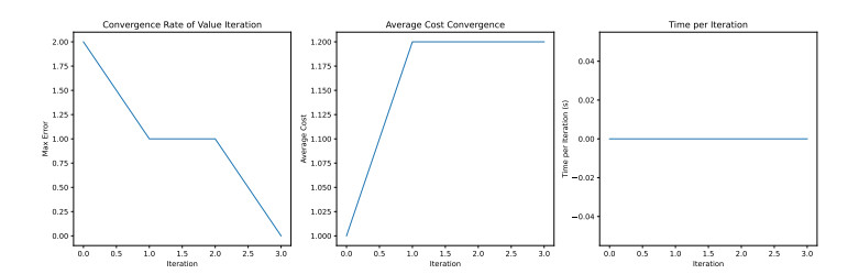
In the context of deterministic discrete-time control systems, we examined the implementation of value iteration (VI) and policy (PI) algorithms in Markov decision processes (MDPs) situated within Borel spaces. The deterministic nature of the system's transfer function plays a pivotal role, as the convergence criteria of these algorithms are deeply interconnected with the inherent characteristics of the probability function governing state transitions. For VI, convergence is contingent upon verifying that the cost difference function stabilizes to a constant $ k $ ensuring uniformity across iterations. In contrast, PI achieves convergence when the value function maintains consistent values over successive iterations. Finally, a detailed example demonstrates the conditions under which convergence of the algorithm is achieved, underscoring the practicality of these methods in deterministic settings.
Citation: Haifeng Zheng, Dan Wang. A study of value iteration and policy iteration for Markov decision processes in Deterministic systems[J]. AIMS Mathematics, 2024, 9(12): 33818-33842. doi: 10.3934/math.20241613
In the context of deterministic discrete-time control systems, we examined the implementation of value iteration (VI) and policy (PI) algorithms in Markov decision processes (MDPs) situated within Borel spaces. The deterministic nature of the system's transfer function plays a pivotal role, as the convergence criteria of these algorithms are deeply interconnected with the inherent characteristics of the probability function governing state transitions. For VI, convergence is contingent upon verifying that the cost difference function stabilizes to a constant $ k $ ensuring uniformity across iterations. In contrast, PI achieves convergence when the value function maintains consistent values over successive iterations. Finally, a detailed example demonstrates the conditions under which convergence of the algorithm is achieved, underscoring the practicality of these methods in deterministic settings.

| [1] | R. Bellman, The theory of dynamic programming, Bull. Amer. Math. Soc., 1954, 503–515. |
| [2] | O. Hernández-Lerma, J. B. Lasserre, Discrete-time Markov control processes: basic optimality criteria, Vol. 30, New York: Springer Science & Business Media, 2012. |
| [3] | O. Hernández-Lerma, J. B. Lasserre, Further topics on discrete-time Markov control processes, Vol. 42, New York: Springer Science & Business Media, 2012. |
| [4] |
O. Hernández-Lerma, L. R. Laura-Guarachi, S. Mendoza-Palacios, A survey of AC problems in deterministic discrete-time control systems, J. Math. Anal. Appl., 522 (2023), 126906. https://doi.org/10.1016/j.jmaa.2022.126906 doi: 10.1016/j.jmaa.2022.126906

|
| [5] | S. P. Meyn, R. L. Tweedie, Markov chains and stochastic stability, 1 Ed., New York: Springer London, 1993. https://doi.org/10.1007/978-1-4471-3267-7 |
| [6] |
W. A. Brock, L. J. Mirman, Optimal economic growth and uncertainty: the discounted case, J. Econ. Theory, 4 (1979), 479–513. https://doi.org/10.4337/9781782543046.00008 doi: 10.4337/9781782543046.00008
|
| [7] |
W. A. Brock, L. J. Mirman, Optimal economic growth and uncertainty: the no discounting case, Int. Econ. Rev., 14 (1973), 560–573. https://doi.org/10.2307/2525969 doi: 10.2307/2525969
|
| [8] | V. Gaitsgory, A. Parkinson, I. Shvartsman, Linear programming based optimality conditions and approximate solution of a deterministic infinite horizon discounted optimal control problem in discrete time, arXiv Preprint, 2017. https://doi.org/10.48550/arXiv.1711.00801 |
| [9] |
O. L. V. Costa, F. Dufour, Average control of Markov decision processes with Feller transition probabilities and general action spaces, J. Math. Anal. Appl., 396 (2012), 58–69. https://doi.org/10.1016/j.jmaa.2012.05.073 doi: 10.1016/j.jmaa.2012.05.073
|
| [10] |
S. P. Meyn, The policy iteration algorithm for average reward Markov decision processes with general state space, IEEE Trans. Automat. Control, 42 (1997), 1663–1680. https://doi.org/10.1109/9.650016 doi: 10.1109/9.650016
|
| [11] | R. Bellman, Dynamic programming, Science, 153 (1966), 34–37. https://doi.org/10.1126/science.153.3731.34 |
| [12] | R. A. Howard, Dynamic programming and markov processes, MIT Press, 1960, 46–69. https://doi.org/10.1086/258477 |
| [13] |
S. Dai, O. Menoukeu-Pamen, An algorithm based on an iterative optimal stopping method for Feller processes with applications to impulse control, perturbation, and possibly zero random discount problems, J. Comput. Appl. Mathe., 421 (2023), 114864. https://doi.org/10.1016/j.cam.2022.114864 doi: 10.1016/j.cam.2022.114864
|
| [14] |
E. A. Feinberg, Y. Liang, On the optimality equation for average cost Markov decision processes and its validity for inventory control, Ann. Ope. Res., 317 (2022), 569–586. https://doi.org/10.1007/s10479-017-2561-9 doi: 10.1007/s10479-017-2561-9
|
| [15] |
Z. Yu, X. Guo, L. Xia, Zero-sum semi-Markov games with state-action-dependent discount factors, Discrete Event Dyn. Syst., 32 (2022), 545–571. https://doi.org/10.1007/s10626-022-00366-4 doi: 10.1007/s10626-022-00366-4
|
| [16] |
S. He, H. Fang, M. Zhang, F. Liu, Z. Ding, Adaptive optimal control for a class of nonlinear systems: the online policy iteration approach, IEEE Trans. Neural Netw. Learn. Syst., 31 (2019), 549–558. https://doi.org/10.1109/TNNLS.2019.2905715 doi: 10.1109/TNNLS.2019.2905715
|
| [17] |
H. Fang, M. Zhang, S. He, X. Luan, F. Liu, Z. Ding, Solving the zero-sum control problem for tidal turbine system: an online reinforcement learning approach, IEEE Trans. Cybern., 53 (2023), 7635–7647. https://doi.org/10.1109/TCYB.2022.3186886 doi: 10.1109/TCYB.2022.3186886
|
| [18] |
H. Fang, Y. Tu, H. Wang, S. He, F. Liu, Z. Ding, et al., Fuzzy-based adaptive optimization of unknown discrete-time nonlinear Markov jump systems with off-policy reinforcement learning, IEEE Trans. Fuzzy Syst., 30 (2022), 5276–5290. https://doi.org/10.1109/TFUZZ.2022.3171844 doi: 10.1109/TFUZZ.2022.3171844
|

Figures(2)

Haifeng Zheng, Dan Wang. A study of value iteration and policy iteration for Markov decision processes in Deterministic systems[J]. AIMS Mathematics, 2024, 9(12): 33818-33842. doi: 10.3934/math.20241613


 DownLoad: