Uplifting edges in higher-order networks: Spectral centralities for non-uniform hypergraphs

Gonzalo Contreras-Aso; Cristian Pérez-Corral; Miguel Romance; Gonzalo Contreras-Aso; Cristian Pérez-Corral; Miguel Romance

doi:10.3934/math.20241539

AIMS Mathematics

2024, Volume 9, Issue 11: 32045-32075. doi: 10.3934/math.20241539

Previous Article Next Article

Research article Special Issues

Uplifting edges in higher-order networks: Spectral centralities for non-uniform hypergraphs

1.
Departamento de Matemática Aplicada, Ciencia e Ingeniería de los Materiales y Tecnología Electrónica, Universidad Rey Juan Carlos, 28933 Móstoles (Madrid), Spain
2.
Laboratorio de Computación Matemática en Redes Complejas y sus Aplicaciones, Universidad Rey Juan Carlos, 28933 Móstoles (Madrid), Spain
3.
Valencian Research Institute for Artificial Intelligence, Universitat Politècnica de València, Camino de Vera, s/n 46022 Valencia, Spain

Received: 09 September 2024 Revised: 21 October 2024 Accepted: 28 October 2024 Published: 11 November 2024
MSC : 05C65, 15A72, 68M10

Spectral analysis of networks states that many structural properties of graphs, such as the centrality of their nodes, are given in terms of their adjacency matrices. The natural extension of such spectral analysis to higher-order networks is strongly limited by the fact that a given hypergraph could have several different adjacency hypermatrices, and hence the results obtained so far are mainly restricted to the class of uniform hypergraphs, which leaves many real systems unattended. A new method for analyzing non-linear eigenvector-like centrality measures of non-uniform hypergraphs was presented in this paper that could be useful for studying properties of $ \mathcal{H} $-eigenvectors and $ \mathcal{Z} $-eigenvectors in the non-uniform case. In order to do so, a new operation——the uplift——was introduced, incorporating auxiliary nodes in the hypergraph to allow for a uniform-like analysis. We later argued why this was a mathematically sound operation, and we furthermore used it to classify a whole family of hypergraphs with unique Perron-like $ \mathcal{Z} $-eigenvectors. We supplemented the theoretical analysis with several examples and numerical simulations on synthetic and real datasets: On the latter, we find a clear improvement over the existing methods, specially in cases where there is a huge disparity between the structure at each order, and on the former, we find that regardless of the chosen uniformization scheme, the nodes were similarly ranked.
- graph theory,
- hypergraphs,
- centrality,
- hypermatrices,
- eigenvectors
Citation: Gonzalo Contreras-Aso, Cristian Pérez-Corral, Miguel Romance. Uplifting edges in higher-order networks: Spectral centralities for non-uniform hypergraphs[J]. AIMS Mathematics, 2024, 9(11): 32045-32075. doi: 10.3934/math.20241539

Related Papers:

Abstract

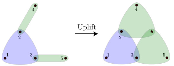
Spectral analysis of networks states that many structural properties of graphs, such as the centrality of their nodes, are given in terms of their adjacency matrices. The natural extension of such spectral analysis to higher-order networks is strongly limited by the fact that a given hypergraph could have several different adjacency hypermatrices, and hence the results obtained so far are mainly restricted to the class of uniform hypergraphs, which leaves many real systems unattended. A new method for analyzing non-linear eigenvector-like centrality measures of non-uniform hypergraphs was presented in this paper that could be useful for studying properties of $ \mathcal{H} $-eigenvectors and $ \mathcal{Z} $-eigenvectors in the non-uniform case. In order to do so, a new operation——the uplift——was introduced, incorporating auxiliary nodes in the hypergraph to allow for a uniform-like analysis. We later argued why this was a mathematically sound operation, and we furthermore used it to classify a whole family of hypergraphs with unique Perron-like $ \mathcal{Z} $-eigenvectors. We supplemented the theoretical analysis with several examples and numerical simulations on synthetic and real datasets: On the latter, we find a clear improvement over the existing methods, specially in cases where there is a huge disparity between the structure at each order, and on the former, we find that regardless of the chosen uniformization scheme, the nodes were similarly ranked.

References

[1]	S. Boccaletti, V. Latora, Y. Moreno, M. Chavez, D. U. Hwang, Complex networks: Structure and dynamics, Phys. Rep., 424 (2006), 175–308. https://doi.org/10.1016/j.physrep.2005.10.009 doi: 10.1016/j.physrep.2005.10.009
[2]	F. Battiston, G. Cencetti, I. Iacopini, V. Latora, M. Lucas, A. Patania, et al., Networks beyond pairwise interactions: Structure and dynamics, Phys. Rep., 874 (2020), 1–92. https://doi.org/10.1016/j.physrep.2020.05.004 doi: 10.1016/j.physrep.2020.05.004
[3]	S. Boccaletti, P. De Lellis, C. del Genio, K. Alfaro-Bittner, R. Criado, S. Jalan, et al., The structure and dynamics of networks with higher-order interactions, Phys. Rep., 1018 (2023), 1–64. https://doi.org/10.1016/j.physrep.2023.04.002 doi: 10.1016/j.physrep.2023.04.002
[4]	Z. K. Zhang, C. Liu, A hypergraph model of social tagging networks, J. Stat. Mech.-Theory E., 2010. https://doi.org/10.1088/1742-5468/2010/10/P10005
[5]	X. L. Liu, C. Zhao, Eigenvector centrality in simplicial complexes of hypergraphs, Chaos Interdisc. J. Nonlinear Sci., 33 (2023). https://doi.org/10.1063/5.0144871 doi: 10.1063/5.0144871
[6]	L. Page, S. Brin, R. Motwani, T. Winograd, The pagerank citation ranking: Bringing order to the web, In: Proceedings of the 7th International World Wide Web Conference, 1998,161–172.
[7]	A. R. Benson, Three hypergraph eigenvector centralities, SIAM J. Math. Data Sci., 1 (2019), 293–312. https://doi.org/10.1137/18M1203031 doi: 10.1137/18M1203031
[8]	L. Q. Qi, Z. Y. Luo, Tensor analysis: Spectral theory and special tensors, Society for Industrial and Applied Mathematics, Philadelphia, PA, 2017.
[9]	D. A. Bini, B. Meini, F. Poloni, On the solution of a quadratic vector equation arising in markovian binary trees, Numer. Linear Algebr., 18 (2011), 981–991. https://doi.org/10.1002/nla.809 doi: 10.1002/nla.809
[10]	L. Q. Qi, Y. J. Wang, E. X. Wu, D-eigenvalues of diffusion kurtosis tensors, J. Comput. Appl. Math., 221 (2008), 150–157. https://doi.org/10.1016/j.cam.2007.10.012 doi: 10.1016/j.cam.2007.10.012
[11]	S. L. Hu, L. Q. Qi, G. F. Zhang, Computing the geometric measure of entanglement of multipartite pure states by means of non-negative tensors, Phys. Rev. A, 93 (2016). https://doi.org/10.1103/PhysRevA.93.012304 doi: 10.1103/PhysRevA.93.012304
[12]	A. R. Benson, D. Gleich, J. Leskovec, Tensor spectral clustering for partitioning higher-order network structures, In: Proceedings of the 2015 SIAM International Conference on Data Mining, 2015,118–126. https://epubs.siam.org/doi/abs/10.1137/1.9781611974010.14
[13]	M. Ng, L. Qi, G. L. Zhou, Finding the largest eigenvalue of a nonnegative tensor, SIAM J. Matrix Anal. A., 31 (2009), 1090–1099. https://doi.org/10.1137/09074838X doi: 10.1137/09074838X
[14]	S. Vigna, Spectral ranking, Cambridge University Press, 2016,433–445. https://doi.org/10.1017/nws.2016.21
[15]	E. Estrada, The structure of complex networks: Theory and applications, Oxford University Press, New York, 2012.
[16]	C. D. Meyer, Matrix analysis and applied linear algebra, SIAM, 2023.
[17]	K. J. Pearson, T. Zhang, On spectral hypergraph theory of the adjacency tensor, Graph. Combinator., 30 (2014), 1233–1248. https://doi.org/10.1007/s00373-013-1340-x doi: 10.1007/s00373-013-1340-x
[18]	K. C. Chang, K. J. Pearson, T. Zhang, Some variational principles for z-eigenvalues of nonnegative tensors, Linear Algebra Appl., 438 (2013), 4166–4182. https://doi.org/10.1016/j.laa.2013.02.013 doi: 10.1016/j.laa.2013.02.013
[19]	A. R. Benson, D. Gleich, Computing tensor $z$-eigenvectors with dynamical systems, SIAM J. Matrix Anal. A., 40 (2019), 1311–1324. https://doi.org/10.1137/18M1229584 doi: 10.1137/18M1229584
[20]	S. G. Aksoy, I. Amburg, S. J. Young, Scalable tensor methods for nonuniform hypergraphs, SIAM J. Math. Data Sci., 6 (2024). https://doi.org/10.1137/23M1584472 doi: 10.1137/23M1584472
[21]	K. C. Chang, T. Zhang, On the uniqueness and non-uniqueness of the positive z-eigenvector for transition probability tensors, J. Math. Anal. Appl., 408 (2013), 525–540. https://doi.org/10.1016/j.jmaa.2013.04.019 doi: 10.1016/j.jmaa.2013.04.019
[22]	K. C. Chang, K. J. Pearson, T. Zhang, Perron-Frobenius theorem for nonnegative tensors, Commun. Math. Sci., 6 (2008), 507–520.
[23]	K. Kovalenko, M. Romance, E. Vasilyeva, D. Aleja, R. Criado, D. Musatov, et al., Vector centrality in hypergraphs, Chaos Soliton. Fract., 162 (2022), 112397. https://doi.org/10.1016/j.chaos.2022.112397 doi: 10.1016/j.chaos.2022.112397
[24]	Y. M. Zhen, J. H. Wang, Community detection in general hypergraph via graph embedding, J. Am. Stat. Assoc., 118 (2022), 1620–1629. https://doi.org/10.1080/01621459.2021.2002157 doi: 10.1080/01621459.2021.2002157
[25]	X. Ouvrard, J. M. Le Goff, S. Marchand-Maillet, Adjacency and tensor representation in general hypergraphs part 1: e-adjacency tensor uniformisation using homogeneous polynomials, arXiv preprint, 2018. https://doi.org/10.48550/arXiv.1712.08189
[26]	A. Banerjee, A. Char, B. Mondal, Spectra of general hypergraphs, Linear Algebra Appl., 518 (2017), 14–30. https://doi.org/10.1016/j.laa.2016.12.022 doi: 10.1016/j.laa.2016.12.022
[27]	N. W. Landry, M. Lucas, I. Iacopini, G. Petri, A. Schwarze, A. Patania, et al., XGI: A Python package for higher-order interaction networks, J. Open Source Softw., 8 (2023). https://doi.org/10.21105/joss.05162
[28]	A. R. Benson, R. Abebe, M. T. Schaub, A. Jadbabaie, J. Kleinberg, Simplicial closure and higher-order link prediction, P. Natl. Acad. Sci., 115 (2018), E11221–E11230. https://doi.org/10.1073/pnas.1800683115 doi: 10.1073/pnas.1800683115
[29]	L. Isella, J. Stehlé, A. Barrat, C. Cattuto, J. F. Pinton, W. Van den Broeck, What's in a crowd? analysis of face-to-face behavioral networks, J. Theor. Biol., 271 (2011), 166–180. https://doi.org/10.1016/j.jtbi.2010.11.033 doi: 10.1016/j.jtbi.2010.11.033
[30]	D. R. Hofstadter, Gödel, Escher, Bach: An Eternal Golden Braid, Basic Books Inc., 1979.
[31]	J. Stehlé, N. Voirin, A. Barrat, C. Cattuto, L. Isella, J. F. Pinton, et al., High-resolution measurements of face-to-face contact patterns in a primary school, PloS One, 6 (2011), e23176. https://doi.org/10.1371/journal.pone.0023176 doi: 10.1371/journal.pone.0023176
[32]	R. Mastrandrea, J. Fournet, A. Barrat, Contact patterns in a high school: A comparison between data collected using wearable sensors, contact diaries and friendship surveys, PloS One, 10 (2015), e0136497. https://doi.org/10.1371/journal.pone.0136497 doi: 10.1371/journal.pone.0136497
[33]	C. Cattuto, W. Van den Broeck, A. Barrat, V. Colizza, J. F. Pinton, A. Vespignani, Dynamics of person-to-person interactions from distributed rfid sensor networks, PloS One, 5 (2010), e11596. https://doi.org/10.1371/journal.pone.0011596 doi: 10.1371/journal.pone.0011596
[34]	K. I. Goh, M. E. Cusick, D. Valle, B. Childs, M. Vidal, A. L. Barabási, The human disease network, P. Natl. Acad. Sci., 104 (2007), 8685–8690. https://doi.org/10.1073/pnas.0701361104 doi: 10.1073/pnas.0701361104
[35]	M. Dewar, J. Healy, X. Pérez-Giménez, P. Prałat, J. Proos, B. Reiniger, et al., Subhypergraphs in non-uniform random hypergraphs, arXiv preprint, 2018. https://doi.org/10.48550/arXiv.1703.07686
[36]	T. G. Kolda, J. R. Mayo, An adaptive shifted power method for computing generalized tensor eigenpairs, SIAM J. Matrix Anal. Appl., 35 (2014), 1563–1581. https://doi.org/10.1137/140951758 doi: 10.1137/140951758
[37]	G. Gallo, G. Longo, S. Pallottino, S. Nguyen, Directed hypergraphs and applications, Discrete Appl. Math., 42 (1993), 177–201. https://doi.org/10.1016/0166-218X(93)90045-P doi: 10.1016/0166-218X(93)90045-P
[38]	G. Contreras-Aso, R. Criado, M. Romance, Beyond directed hypergraphs: Heterogeneous hypergraphs and spectral centralities, J. Complex Netw., 12 (2024), cnae037. https://doi.org/10.1093/comnet/cnae037 doi: 10.1093/comnet/cnae037
[39]	J. L. Guo, X. Y. Zhu, Q. Suo, J. Forrest, Non-uniform evolving hypergraphs and weighted evolving hypergraphs, Sci. Rep., 6 (2016), 36648. https://doi.org/10.1038/srep36648 doi: 10.1038/srep36648

Reader Comments

Your name:*

Email:*
© 2024 the Author(s), licensee AIMS Press. This is an open access article distributed under the terms of the Creative Commons Attribution License (http://creativecommons.org/licenses/by/4.0)