Analytical discovery of dark soliton lattices in (2+1)-dimensional generalized fractional Kundu-Mukherjee-Naskar equation

Abdulah A. Alghamdi; Abdulah A. Alghamdi

doi:10.3934/math.20241123

AIMS Mathematics

2024, Volume 9, Issue 8: 23100-23127. doi: 10.3934/math.20241123

Previous Article Next Article

Research article Special Issues

Analytical discovery of dark soliton lattices in (2+1)-dimensional generalized fractional Kundu-Mukherjee-Naskar equation

Abdulah A. Alghamdi ^{1,2
,
,}

1.
Mathematical Modeling and Applied Computation (MMAC) Research Group, Department of Mathematics, King Abdulaziz University, Jeddah-21589, Saudi Arabia
2.
Center of Modern Mathematical Sciences and their Applications (CMMSA), King Abdulaziz, University, Jeddah-21589, Saudi Arabia

Received: 10 June 2024 Revised: 07 July 2024 Accepted: 15 July 2024 Published: 29 July 2024

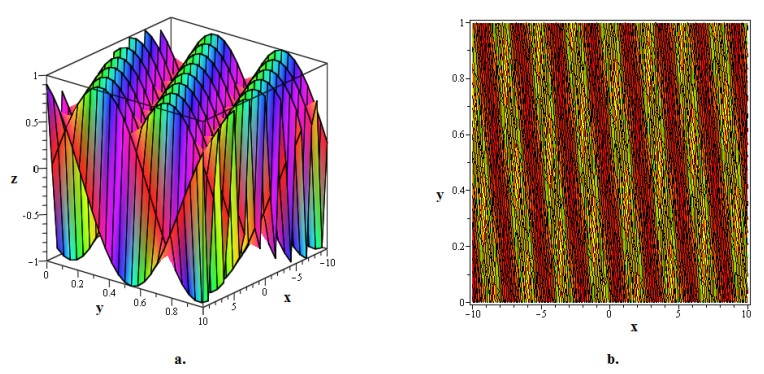
This research explored optical soliton solutions for the (2+1)-dimensional generalized fractional Kundu-Mukherjee-Naskar equation (gFKMNE), which is a nonlinear model for explaining pulse transmission in communication structures and optical fibers. Two enhanced variants of $(\frac{G'}{G})$ -expansion method were employed, namely, extended $(\frac{G'}{G})$ -expansion method and the generalized $(r+\frac{G'}{G})$ -expansion method, based on the wave transformation of the model into integer-order nonlinear ordinary differential equations (NODEs). By assuming a series-form solution for the resultant NODEs, these strategic methods further translated them into a system of nonlinear algebraic equations. Solving these equations provided optical soliton solutions for gFKMNE using the Maple-13 tool. Through 3D and contour visuals, it was revealed that the constructed soliton solutions are periodically arranged in the optical medium, forming dark soliton lattices. These dark soliton lattices are significant in several domains, such as optical signal processing, optical communications, and nonlinear optics.

Keywords:

Citation: Abdulah A. Alghamdi. Analytical discovery of dark soliton lattices in (2+1)-dimensional generalized fractional Kundu-Mukherjee-Naskar equation[J]. AIMS Mathematics, 2024, 9(8): 23100-23127. doi: 10.3934/math.20241123

Related Papers:

[1]	Naher Mohammed A. Alsafri . Solitonic behaviors in the coupled Drinfeld-Sokolov-Wilson system with fractional dynamics. AIMS Mathematics, 2025, 10(3): 4747-4774. doi: 10.3934/math.2025218
[2]	Chun Huang, Zhao Li . Soliton solutions of conformable time-fractional perturbed Radhakrishnan-Kundu-Lakshmanan equation. AIMS Mathematics, 2022, 7(8): 14460-14473. doi: 10.3934/math.2022797
[3]	Ghazala Akram, Saima Arshed, Maasoomah Sadaf, Hajra Mariyam, Muhammad Nauman Aslam, Riaz Ahmad, Ilyas Khan, Jawaher Alzahrani . Abundant solitary wave solutions of Gardner's equation using three effective integration techniques. AIMS Mathematics, 2023, 8(4): 8171-8184. doi: 10.3934/math.2023413
[4]	Imran Siddique, Khush Bukht Mehdi, Sayed M Eldin, Asim Zafar . Diverse optical solitons solutions of the fractional complex Ginzburg-Landau equation via two altered methods. AIMS Mathematics, 2023, 8(5): 11480-11497. doi: 10.3934/math.2023581
[5]	Naeem Ullah, Muhammad Imran Asjad, Jan Awrejcewicz, Taseer Muhammad, Dumitru Baleanu . On soliton solutions of fractional-order nonlinear model appears in physical sciences. AIMS Mathematics, 2022, 7(5): 7421-7440. doi: 10.3934/math.2022415
[6]	Musarat Bibi, Salah Mahmoud Boulaaras, Patricia J.Y. Wong, Muhammad Shoaib Saleem . Exploring families of soliton solutions for the fractional Akbota equation in optical fiber telecommunication systems. AIMS Mathematics, 2025, 10(5): 12254-12285. doi: 10.3934/math.2025555
[7]	Haitham Qawaqneh, Ali Altalbe, Ahmet Bekir, Kalim U. Tariq . Investigation of soliton solutions to the truncated M-fractional (3+1)-dimensional Gross-Pitaevskii equation with periodic potential. AIMS Mathematics, 2024, 9(9): 23410-23433. doi: 10.3934/math.20241138
[8]	Emad H. M. Zahran, Omar Abu Arqub, Ahmet Bekir, Marwan Abukhaled . New diverse types of soliton solutions to the Radhakrishnan-Kundu-Lakshmanan equation. AIMS Mathematics, 2023, 8(4): 8985-9008. doi: 10.3934/math.2023450
[9]	Mahmoud Soliman, Hamdy M. Ahmed, Niveen Badra, M. Elsaid Ramadan, Islam Samir, Soliman Alkhatib . Influence of the $ \beta $-fractional derivative on optical soliton solutions of the pure-quartic nonlinear Schrödinger equation with weak nonlocality. AIMS Mathematics, 2025, 10(3): 7489-7508. doi: 10.3934/math.2025344
[10]	Noor Alam, Mohammad Safi Ullah, Jalil Manafian, Khaled H. Mahmoud, A. SA. Alsubaie, Hamdy M. Ahmed, Karim K. Ahmed, Soliman Al Khatib . Bifurcation analysis, chaotic behaviors, and explicit solutions for a fractional two-mode Nizhnik-Novikov-Veselov equation in mathematical physics. AIMS Mathematics, 2025, 10(3): 4558-4578. doi: 10.3934/math.2025211

Abstract

1. Introduction

In numerous engineering and scientific domains, nonlinear fractional partial differential equations (NFDEs) have gained significant importance in the description and modelling of intricate processes. The memory and inherited characteristics of the system being modelled can be precisely captured via NFPDEs. These equations are particularly helpful for explaining anomalous diffusion phenomena and have a wide range of applications in disciplines like chemistry, physics, engineering, finance, biology, and economics ^{[1,2,3,4,5,6]}. As a result, in many application domains, the exploration of NFPDEs is crucial to comprehending and forecasting the behavior of complex systems. Nonetheless, there are special difficulties in resolving and interpreting fractional derivatives due to their non-locality and non-linearity. The solution and analysis of these equations may require the development of new methods and tools, as traditional analytical and numerical approaches might not be directly relevant. Notwithstanding these difficulties, research on NFPDEs has produced significant advances in a number of scientific and engineering domains ^[7,8,9]. Research opportunities have increased and our understanding of complicated processes has improved as a result of the development of new analytical and numerical techniques for solving and analyzing NFPDEs ^[10,11,12]. Exact solutions to nonlinear fractional problems can currently be obtained by a variety of effective methods, such as the generalized projective Riccati equation approach ^[13], sine-Gordon expansion method ^[14], generalized Riccati method and the auxiliary ordinary differential equation method ^[15], Lie symmetry approach ^[16], first integral method ^[17], modified Kudryashov method ^[18], extended exp ${(-\phi(\xi))}$ -expansion method ^[19], modified auxiliary equation method ^[20], unified method ^[21], $(\frac{G'}{G})$ -expansion methods ^[22,23,24], Khater methods ^[25,26], Poincaré-Lighthill-Kuo method ^[27], Riccati-Bernoulli Sub-ODE ^[28], exp-function method ^[29], fractional Sin-Gordon method ^[30], sub-equation method ^[31], tanh-method ^[32], extended direct algebraic method ^{[33,34,35,36]}, Sardar sub-equation method ^[37], exponential rational function method ^[38], and so on ^{[39,40,41,42,43,44]}.

Kundu et al. ^[45] introduced the Kundu-Mukherjee-Naskar equation (KMNE) for the first time in $2014$ and found optical soliton solutions for it. The KMNE has been the subject of extensive research recently. Its wave events are crucial for accurately modelling propagation pulses in high-speed data transfer in communication systems, optical fibers and the ocean currents of rogue waves ^[46,47,48]. One common application for optical fibers is the transmission of light between their two ends. Their long-distance and faster data transmission rate compared to wires makes them commonly employed in optical fiber communications. The goal of the current study is to construct and analyze optical soliton solutions for the gFKMNE, a fractional generalization of KMNE, which exhibits the following dimensionless display ^[49]:

$\begin{equation} i D^{\delta}_{t}z+a D^{\beta}_{y}(D^{\alpha}_{x} z)+i b z(z D^{\alpha}_{x} z^{*}-z^{*} D^{\alpha}_{x}) = 0, \end{equation}$

(1.1)

wherein $0 < \alpha, \beta, \delta \leq1$ , $z = z(t, x, y)$ is the quantity that represents a complex wave envelope, $z^{*}$ is the complex conjugate of $z$ . Furthermore, the dispersion term and the nonlinearity term are indicated by the two parameters $a$ , $b$ respectively. The wave's temporal history is represented by the first term in Eq (1), which is succeeded by the dispersion term $a D^{\beta}_{y}(D^{\alpha}_{x} z)$ . Ultimately, the coefficient of $b$ that is changed from the standard Kerr law nonlinearity represents the nonlinear portion. In optical fibers and communication systems, the pulse propagation is described by this equation. The fractional derivatives $D^{\alpha}_{x}(\circ)$ , $D^{\beta}_{y}(\circ)$ , and $D^{\delta}_{t}(\circ)$ are the generalized conformable fractional derivatives (gCFDs) of order $\alpha$ , $\beta$ , and $\delta$ respectively.

In many applications, such as irrigation and river flows, tidal waves, weather research and tsunami prediction, Eq (1.1) is used. Due to such significance, many researchers have developed an interest in examining Eq (1.1). For instance, Eq (1.1) was solved with new exact solutions by Günerhan et al. ^[50] through the use of an enhanced direct algebraic approach. Using the csch-approach, extended tanh-coth method, and extended rational sinh-cosh method, Rizvi et al. ^[51] were able to get the singular soliton, dark soliton, combination dark-singular soliton, and other hyperbolic solutions for Eq (1.1). Talarposhti et al. ^[52] derived optical soliton solutions for the KMNE using the exp-function approach. Onder et al. ^[53] used the novel Kudryashov techniques along with the Sardar sub-equation to introduce optical soliton solutions for the KMNE. Zafar et al. ^[54] found new soliton solutions for the KMNE by employing the exp-function approach and the extended Jacobi's elliptic expansion function. Kumar et al. ^[55] used the new auxiliary equation approach with the generalized Kudryashov method to find dark, bright, periodic U-shaped, and singular soliton solutions for Eq (1.1). Furthermore, this equation was investigated by other authors through the use of new precise solution techniques such the semi-inverse approach ^[56], the extended trial function method ^[57], the sine-Gordon and sinh-Gordon expansion methods ^[58], the Hamiltonian-based algorithm ^[59], Laplace-Adomian decomposition method ^[60], and other methods ^{[61,62,63,64,65]}.

Inspired by current research, we seek to address gFKMNE expressed in (1.1) through two enhanced implementations of the $(\frac{G'}{G})$ -expansion technique: the extended $(\frac{G'}{G})$ -expansion method and the generalized $(r+\frac{G'}{G})$ -expansion method, which are based on the reduction of NFPDEs to integer-order NODEs produced by the model's wave transformation. The strategic techniques further transform the resultant NODEs into an algebraic system of nonlinear equations by assuming a series-form solution. These equations may then be solved using the Maple tool to produce dark soliton lattices for gFKMNE. The important solitons in these dark soliton lattices are organized regularly in an optical medium. Dark soliton formations are collections of dark solitaires arranged regularly inside a medium. They are frequently shaped like wave channels or optical fibers. Similar to the lattice of a crystal, these solitons are restricted to areas of decreased optical intensity within a larger field that retain their structure and amplitude while moving. Not only can dark soliton lattices be used to precisely control and manipulate optical waves, but they can also be used to process information and communications networks, provide insight into nonlinear optics phenomena, provide platforms for basic research on the behavior of wave propagation, and have potential applications in signal processing, optical communication, and sensing. Thus, dark soliton lattices offer a stimulating new topic for nonlinear optics research that will enable both basic and applied investigations ^[66,67,68].

The format of the present article is as follows: Section 1 provides an introduction. The operational mechanism for the $(\frac{G'}{G})$ -expansion methods and the description of gCFD are detailed in Section 2. We build many additional sets of optical soliton solutions for Eq (1.1) in Section 3. A few illustrations and a graphical representations of dark soliton lattices are presented and discussed in Section 4. Our study excursion comes to an end with the provided conclusion in Section 5.

2. Materials and methodology

In this section, the basic definition of used fractional derivative gCFD and the operational procedure of the proposed methods are presented.

2.1. The definition of gCFD

Explicit soliton solutions to nonlinear FPDEs can be obtained by taking use of the advantages that gCFDs have over conventional fractional derivative operators. Notably, alternate formulations of fractional derivatives do not provide the optical soliton solutions of Eq (1.1) because they violate the chain rule ^[69,70]. Consequently, gCFDs were added to Eq (1.1). ^[71] defined this derivative operator of order $\wp$ as follows:

$\begin{equation} ^{gCFD} D^\wp_\varphi z(\varphi) = \lim\limits_{\varpi \to 0} \frac{z( (\frac{\Gamma(n)}{\Gamma(n-\wp+1)})\varpi \varphi^{1-\wp}+\varphi)-z(\varphi)}{\varpi}, \quad \wp \in (0,1] \quad n \geq -1, \quad n \in R. \end{equation}$

(2.1)

We utilize the following characteristics of this derivative in this study:

$\begin{equation} ^{gCFD} D^\wp_\varphi \varphi^\gamma = \frac{\gamma \Gamma(n)}{\Gamma(n-\wp+1)} \varphi^{\gamma-\wp}, \quad \forall \gamma \in R, \end{equation}$

(2.2)

$\begin{equation} ^{gCFD} D^\wp_\varphi(\gamma_1\rho(\varphi)\pm \gamma_2\eta(\varphi)) = \gamma_1 {^{gCFD} D^\wp_\varphi(\rho(\varphi))}\pm \gamma_2 {^{gCFD} D^\wp_\varphi(\eta(\varphi))}, \end{equation}$

(2.3)

$\begin{equation} ^{gCFD} D^\wp_\varphi \omega[\zeta(\varphi)] = \omega'_\zeta(\zeta(\varphi)) {^{gCFD} D^\wp_\varphi \zeta(\varphi)} , \end{equation}$

(2.4)

where $\rho(\varphi)$ , $\eta(\varphi)$ , $\omega(\varphi)$ , and $\zeta(\varphi)$ are arbitrary differentiable functions, whereas $\gamma$ , $\gamma_1$ and $\gamma_2$ signify constants.

2.2. The working methodology of $(\frac{G'}{G})$ -expansion method

In this phase of our study, we discuss the processes of the $(\frac{G'}{G})$ -expansion approach, with a focus on solving the given general NFPDE:

$\begin{equation} R(z, D^{ \delta}_{t} z, D^{ \alpha}_{x_1}z, D^{ \beta}_{x_1} z,z D^{ \alpha}_{x_1} z, \ldots) = 0, \quad 0 < \alpha, \beta , \delta \leq1, \end{equation}$

(2.5)

where $z = z(t, x_1, x_2, x_3, \ldots, x_j)$ .

Equation (2.5) is solved using the following strategy:

(ⅰ). Starting with a variable transformation of the framework $z(t, x_1, x_2, x_3, \dots, x_j) = Z(\varphi)$ , where $\varphi$ can be stated in a number of ways. Equation (2.5) progresses via this transformation, resulting in the NODE that follows:

$\begin{equation} Q(Z,Z'Z,Z',\dots) = 0, \end{equation}$

(2.6)

where $Z' = \frac{d Z}{d\varphi}$ . On rare occasions, the NODE may become vulnerable to the homogeneous balancing principle due to the integration of Eq (2.6).

(ⅱ). Next, based on the method's version, we assume the following series-form solution for (2.6):

Version 1. For the extended $(\frac{G'}{G})$ -expansion method, we assume the following $(\frac{G'}{G})$ solution:

$\begin{equation} Z(\varphi) = \sum\limits_{l = -\rho}^{\rho}\tau_l(\frac{G'(\varphi)}{G(\varphi)})^l, \end{equation}$

(2.7)

Version 2. For the generalized $(r+\frac{G'}{G})$ -expansion method, we assume the following $(\frac{G'}{G})$ solution:

$\begin{equation} Z(\varphi) = \sum\limits_{l = -\rho}^{\rho}\tau_l(r+\frac{G'(\varphi)}{G(\varphi)})^l, \quad r \in R, \end{equation}$

(2.8)

where it is subsequently necessary to compute the values of $\tau_l's (l = -\rho... \rho)$ . The balance number $\rho$ , a positive integer in Eqs (2.7) and (2.8), can be found by homogeneously balancing the nonlinear terms and the derivative with the highest order terms in Eq (2.6). Greater accuracy can be achieved in determining the balance number $\rho$ by applying the following mathematical formulas:

$\begin{equation} D(\frac{d^p Z}{d\varphi^p}) = \rho+p, \ \ \text{and} \ \ D(Z^q (\frac{d^p Z}{d\varphi^p})^s) = \rho q+p(s+\rho), \end{equation}$

(2.9)

where $D$ expresses the degree of $Z(\varphi)$ , whereas $p, q$ , and $s$ are positive integers.

Moreover, the function $G(\varphi)$ in Eq (2.8) satisfies the subsequent second-order linear ODE:

$\begin{equation} G''(\varphi)+\lambda G'(\varphi)+\mu G(\varphi) = 0, \end{equation}$

(2.10)

where $\lambda, \mu$ are constants.

Moreover, with Eq (2.10)'s general solution, we have:

$\begin{equation} \bigg(\frac{G'(\varphi)}{G(\varphi)}\bigg) = \left\{ \begin{array}{ll} \frac{1}{2}\,{\frac {\sqrt {\kappa} \left( \nu_{{1}}\sinh \left( \frac{1}{2}\,\sqrt { \kappa}\varphi \right) +\nu_{{2}}\cosh \left( \frac{1}{2}\,\sqrt {\kappa}\varphi \right) \right) }{\nu_{{1}}\cosh \left( \frac{1}{2}\,\sqrt {\kappa}\varphi \right) +\nu_{{2}}\sinh \left( \frac{1}{2}\,\sqrt {\kappa}\varphi \right) }}-\frac{1}{2} \,\lambda, & \kappa < 0, \\ \frac{1}{2}\,{\frac {\sqrt {-\kappa} \left( -\nu_{{1}}\sin \left( \frac{1}{2}\,\sqrt {- \kappa}\varphi \right) +\nu_{{2}}\cos \left( \frac{1}{2}\,\sqrt {-\kappa}\varphi \right) \right) }{\nu_{{1}}\cos \left( \frac{1}{2}\,\sqrt {-\kappa}\varphi \right) +\nu_{{2}}\sin \left( \frac{1}{2}\,\sqrt {-\kappa}\varphi \right) }}-\frac{1}{2} \,\lambda, & \kappa > 0, \\ {\frac {\nu_{{2}}}{\nu_{{1}}+\nu_{{2}}\varphi}}, & \kappa = 0,\\ \end{array} \right. \end{equation}$

(2.11)

where $\kappa = \lambda^2-4\mu$ , while $\nu_1$ and $\nu_2$ in (2.11) are arbitrary constants.

(ⅲ). Next, we insert Eqs (2.8) or (2.7) into Eq (2.6) or into the Equation that we acquired from the integration of Eq (2.6), and we gather all the terms that have an analogous power of $(\frac{G'(\varphi)}{G(\varphi)})$ .

(ⅳ). The derived polynomial $(\frac{G'(\varphi)}{G(\varphi)})^i$ has all of its coefficients equal to zero, resulting in a collection of nonlinear algebraic equations in $\tau_l (l = -\rho..., \rho)$ , $\lambda$ , $\mu$ , and other necessary parameters.

(ⅴ). The unresolved parameters are discovered by using the Maple tool to solve the resulting system.

(ⅵ). To generate sets of soliton solutions for Eq (2.5), the values predicted from step 5 are subsequently substituted in Eqs (2.7) or (2.8), depending on the version.

3. Establishing optical soliton solutions for gFKMNE

We use the suggested methods in this section to build families of optical soliton solutions for (1.1). Using the subsequent wave modification as a component of the procedure, we can (1.1):

$\begin{equation} \begin{split} &z(x,y,t) = e^{i \xi} Z(\varphi),\quad \xi = \xi(t,x,y), \quad \varphi = \varphi(t,x,y), \\ & \varphi = {\frac {p_{{1}}\Gamma \left( n-\alpha+1 \right) {x}^{\alpha}}{\alpha \,\Gamma \left( n \right) }}+{\frac {p_{{2}}\Gamma \left( n-\beta+1 \right) {y}^{\beta}}{\beta\,\Gamma \left( n \right) }}-{\frac {\varrho\, \Gamma \left( n-\delta+1 \right) {t}^{\delta}}{\delta\,\Gamma \left( n \right) }}, \\ & \xi = -{\frac {q_{{1}}\Gamma \left( n-\alpha+1 \right) {x}^{\alpha}}{\alpha \,\Gamma \left( n \right) }}-{\frac {q_{{2}}\Gamma \left( n-\beta+1 \right) {y}^{\beta}}{\beta\,\Gamma \left( n \right) }}+{\frac { \omega\,\Gamma \left( n-\delta+1 \right) {t}^{\delta}}{\delta\, \Gamma \left( n \right) }}+\theta_{{0}}, \\ \end{split} \end{equation}$

(3.1)

where $Z(\varphi)$ symbolizes the amplitude part, $q_1$ and $q_2$ indicate wave numbers in the $x-$ and $y-$ directions, respectively, $\omega$ represents the frequency of the wave and $\theta_0$ is a constant, the parameters $p_1$ and $p_2$ indicate inverse width along the $x$ and $y$ directions, respectively, and $\varrho$ is used for the velocity, delivering the afterwards NODE from the real part of (1.1):

$\begin{equation} \begin{split} - a p_1 p_2 Z''-(\omega+a q_1 q_2) Z -2 b q_1 Z^3 = 0, \end{split} \end{equation}$

(3.2)

with the constraint from the imaginary part:

$\begin{equation} \varrho = -a \left( q_{{1}}p_{{2}}+q_{{2}}p_{{1}} \right). \end{equation}$

(3.3)

It is established that $\rho = 1$ when a homogeneous balancing condition between $Z''$ and $Z^3$ (given in (3.2)) has been created.

3.1. Implementation of the extended $(\frac{G'}{G})$ -expansion method

First, we wish to address (3.2) with the help of the extended $(\frac{G'}{G})$ -expansion method. Equation (2.7) yields the following closed form solution for (3.2) when $\rho = 1$ is substituted in it:

$\begin{equation} U(\varphi) = \sum\limits_{l = -1}^{1}\tau_l \bigg(\frac{G'(\varphi)}{G(\varphi)}\bigg)^l. \end{equation}$

(3.4)

By including (3.4) in (3.2) and bringing together terms with a comparable power of $\bigg(\frac{G'(\varphi)}{G(\varphi)}\bigg)$ , we get an expression based on the terms $\bigg(\frac{G'(\varphi)}{G(\varphi)}\bigg)$ . By setting the coefficients to zero, this formula can be converted into a set of algebraic nonlinear equations. The system can be solved using Maple in the following three cases of solutions:

Case 1.1.

$\begin{equation} \begin{split} &\tau_{{0}} = \frac{1}{2}\,{\frac {\tau_{{-1}}\lambda}{\mu}},\tau_{{1}} = 0,\tau_{ {-1}} = \tau_{{-1}},p_{{1}} = p_{{1}},p_{{2}} = p_{{2}},q_{{1}} = {\frac {ap_{ {1}}p_{{2}}{\mu}^{2}}{b{\tau_{{-1}}}^{2}}},\\ &q_{{2}} = q_{{2}},\omega = -\frac{1}{2} \,{\frac {ap_{{1}}p_{{2}} \left( -4\,\mu\,b{\tau_{{-1}}}^{2}+2\,a{\mu} ^{2}q_{{2}}+{\lambda}^{2}b{\tau_{{-1}}}^{2} \right) }{b{\tau_{{-1}}}^{ 2}}}. \end{split} \end{equation}$

(3.5)

Case 1.2.

$\begin{equation} \begin{split} &\tau_{{0}} = \frac{1}{2}\,\tau_{{1}}\lambda,\tau_{{1}} = \tau_{{1}},\tau_{{-1}} = 0 ,p_{{1}} = p_{{1}},p_{{2}} = p_{{2}},q_{{1}} = {\frac {ap_{{1}}p_{{2}}}{b{ \tau_{{1}}}^{2}}},\\ &q_{{2}} = q_{{2}},\omega = -\frac{1}{2}\,{\frac {ap_{{1}}p_{{2}} \left( -4\,\mu\,b{\tau_{{1}}}^{2}+2\,aq_{{2}}+{\lambda}^{2}b{\tau_{{1 }}}^{2} \right) }{b{\tau_{{1}}}^{2}}}. \end{split} \end{equation}$

(3.6)

Case 1.3.

$\begin{equation} \begin{split} \tau_{{0}} = \tau_{{0}},\tau_{{1}} = \tau_{{1}},\tau_{{-1}} = \tau_{{-1}},p _{{1}} = 0,p_{{2}} = p_{{2}},q_{{1}} = 0,q_{{2}} = q_{{2}},\omega = 0. \end{split} \end{equation}$

(3.7)

Considering case 1.1 and utilizing Eq (3.1), (3.4) and the corresponding general solution of (2.10), we construct the subsequent plethora of optical soliton solutions for (1.1):

Family 1.1.1. When $\tau > 0$ ,

(ⅰ) When $\nu_1\neq0$ , $\nu_2\neq0$

$\begin{equation} \begin{split} u_{1,1,1}(t,x,y) = & e^{i \xi}\bigg( \tau_{{-1}} \left( \frac{1}{2}\,{\frac {\sqrt {\kappa} \left( \nu_{{1}}\sinh \left( \frac{1}{2}\,\sqrt {\kappa}\varphi \right) +\nu_{{2}}\cosh \left( \frac{1}{2} \,\sqrt {\kappa}\varphi \right) \right) }{\nu_{{1}}\cosh \left( \frac{1}{2} \,\sqrt {\kappa}\varphi \right) +\nu_{{2}}\sinh \left( \frac{1}{2}\,\sqrt { \kappa}\varphi \right) }}-\frac{1}{2}\,\lambda \right) ^{-1}+\frac{1}{2}\,{\frac { \tau_{{-1}}\lambda}{\mu}} \bigg). \end{split} \end{equation}$

(3.8)

(ⅱ) When $\nu_1 = 0$ , $\nu_2\neq0$

$\begin{equation} \begin{split} u_{1,1,2}(t,x,y) = & e^{i \xi}\bigg( {\frac {\tau_{{-1}}}{\frac{1}{2}\,\sqrt {\kappa}\coth \left( \frac{1}{2}\,\sqrt { \kappa}\varphi \right) -\frac{1}{2}\,\lambda}}+\frac{1}{2}\,{\frac {\tau_{{-1}} \lambda}{\mu}} \bigg). \end{split} \end{equation}$

(3.9)

(ⅲ) When $\nu_1\neq0$ , $\nu_2 = 0$

$\begin{equation} \begin{split} u_{1,1,3}(t,x,y) = & e^{i \xi}\bigg( {\frac {\tau_{{-1}}}{\frac{1}{2}\,\sqrt {\kappa}\tanh \left( \frac{1}{2}\,\sqrt { \kappa}\varphi \right) -\frac{1}{2}\,\lambda}}+\frac{1}{2}\,{\frac {\tau_{{-1}} \lambda}{\mu}} \bigg). \end{split} \end{equation}$

(3.10)

Family 1.1.2. When $\tau < 0$ ,

(ⅰ) When $\nu_1\neq0$ , $\nu_2\neq0$

$\begin{equation} \begin{split} u_{1,1,4}(t,x,y) = & e^{i \xi}\bigg( \tau_{{-1}} \left( \frac{1}{2}\,{\frac {\sqrt {-\kappa} \left( -\nu_{{1}}\sin \left( \frac{1}{2}\,\sqrt {-\kappa}\varphi \right) +\nu_{{2}}\cos \left( \frac{1}{2} \,\sqrt {-\kappa}\varphi \right) \right) }{\nu_{{1}}\cos \left( \frac{1}{2} \,\sqrt {-\kappa}\varphi \right) +\nu_{{2}}\sin \left( \frac{1}{2}\,\sqrt {- \kappa}\varphi \right) }}-\frac{1}{2}\,\lambda \right) ^{-1}+\frac{1}{2}\,{\frac { \tau_{{-1}}\lambda}{\mu}} \bigg). \end{split} \end{equation}$

(3.11)

(ⅱ) When $\nu_1 = 0$ , $\nu_2\neq0$

$\begin{equation} \begin{split} u_{1,1,5}(t,x,y) = & e^{i \xi}\bigg( {\frac {\tau_{{-1}}}{\frac{1}{2}\,\sqrt {-\kappa}\cot \left( \frac{1}{2}\,\sqrt {- \kappa}\varphi \right) -\frac{1}{2}\,\lambda}}+\frac{1}{2}\,{\frac {\tau_{{-1}} \lambda}{\mu}} \bigg). \end{split} \end{equation}$

(3.12)

(ⅲ) When $\nu_1\neq0$ , $\nu_2 = 0$

$\begin{equation} \begin{split} u_{1,1,6}(t,x,y) = & e^{i \xi}\bigg( {\frac {\tau_{{-1}}}{-\frac{1}{2}\,\sqrt {-\kappa}\tan \left( \frac{1}{2}\,\sqrt {- \kappa}\varphi \right) -\frac{1}{2}\,\lambda}}+\frac{1}{2}\,{\frac {\tau_{{-1}} \lambda}{\mu}} \bigg). \end{split} \end{equation}$

(3.13)

Family 1.1.3. When $\tau = 0$ ,

(ⅰ) When $\nu_1\neq0$ , $\nu_2\neq0$

$\begin{equation} \begin{split} u_{1,1,7}(t,x,y) = & e^{i \xi}\bigg({\frac {\tau_{{-1}} \left( \nu_{{1}}+\nu_{{2}}\varphi \right) }{\nu_{ {2}}}}+\frac{1}{2}\,{\frac {\tau_{{-1}}\lambda}{\mu}} \bigg). \end{split} \end{equation}$

(3.14)

(ⅱ) When $\nu_1 = 0$ , $\nu_2\neq0$

$\begin{equation} \begin{split} u_{1,1,8}(t,x,y) = & e^{i \xi}\bigg( {\frac {\tau_{{-1}}}{{\varphi }^{-1}-\frac{1}{2}\,\lambda}}+\frac{1}{2}\,{\frac {\tau_ {{-1}}\lambda}{\mu}} \bigg). \end{split} \end{equation}$

(3.15)

(ⅲ) When $\nu_1\neq0$ , $\nu_2 = 0$

$\begin{equation} \begin{split} u_{1,1,9}(t,x,y) = & e^{i \xi}\bigg( -2\,{\frac {\tau_{{-1}}}{\lambda}}+\frac{1}{2}\,{\frac {\tau_{{-1}}\lambda}{ \mu}} \bigg), \end{split} \end{equation}$

(3.16)

where $\varphi = {\frac {p_{{1}}\Gamma \left(n-\alpha+1 \right) {x}^{\alpha}}{\alpha \, \Gamma \left(n \right) }}+{\frac {p_{{2}}\Gamma \left(n-\beta+1 \right) {y}^{\beta}}{\beta\, \Gamma \left(n \right) }}-{\frac {\varrho\, \Gamma \left(n-\delta+1 \right) {t}^{\delta}}{\delta\, \Gamma \left(n \right) }}$ $\xi = -{\frac {q_{{1}}\Gamma \left(n-\alpha+1 \right) {x}^{\alpha}}{\alpha \, \Gamma \left(n \right) }}-{\frac {q_{{2}}\Gamma \left(n-\beta+1 \right) {y}^{\beta}}{\beta\, \Gamma \left(n \right) }}+{\frac { \omega\, \Gamma \left(n-\delta+1 \right) {t}^{\delta}}{\delta\, \Gamma \left(n \right) }}+\theta_{{0}}$ for $q_1$ and $\omega$ defined in Eq (3.5).

Considering case 1.2 and utilizing Eq (3.1), (3.4) and the corresponding general solution of (2.10), we construct the subsequent plethora of optical soliton solutions for (1.1):

Family 1.2.1. When $\tau > 0$ ,

(ⅰ) When $\nu_1\neq0$ , $\nu_2\neq0$

$\begin{equation} \begin{split} u_{1,2,1}(t,x,y) = & e^{i \xi}\bigg( \frac{1}{2}\,\tau_{{1}}\lambda+\tau_{{1}} \left( \frac{1}{2}\,{\frac {\sqrt {\kappa} \left( \nu_{{1}}\sinh \left( \frac{1}{2}\,\sqrt {\kappa}\varphi \right) +\nu _{{2}}\cosh \left( \frac{1}{2}\,\sqrt {\kappa}\varphi \right) \right) }{\nu_ {{1}}\cosh \left( \frac{1}{2}\,\sqrt {\kappa}\varphi \right) +\nu_{{2}}\sinh \left( \frac{1}{2}\,\sqrt {\kappa}\varphi \right) }}-\frac{1}{2}\,\lambda \right) \bigg). \end{split} \end{equation}$

(3.17)

(ⅱ) When $\nu_1 = 0$ , $\nu_2\neq0$

$\begin{equation} \begin{split} u_{1,2,2}(t,x,y) = & e^{i \xi}\bigg( \frac{1}{2}\,\tau_{{1}}\lambda+\tau_{{1}} \left( \frac{1}{2}\,\sqrt {\kappa}\coth \left( \frac{1}{2}\,\sqrt {\kappa}\varphi \right) -\frac{1}{2}\,\lambda \right) \bigg). \end{split} \end{equation}$

(3.18)

(ⅲ) When $\nu_1\neq0$ , $\nu_2 = 0$

$\begin{equation} \begin{split} u_{1,2,3}(t,x,y) = & e^{i \xi}\bigg( \frac{1}{2}\,\tau_{{1}}\lambda+\tau_{{1}} \left( \frac{1}{2}\,\sqrt {\kappa}\tanh \left( \frac{1}{2}\,\sqrt {\kappa}\varphi \right) -\frac{1}{2}\,\lambda \right) \bigg). \end{split} \end{equation}$

(3.19)

Family 1.2.2. When $\tau < 0$ ,

(ⅰ) When $\nu_1\neq0$ , $\nu_2\neq0$

$\begin{equation} \begin{split} u_{1,2,4}(t,x,y) = & e^{i \xi}\bigg( \frac{1}{2}\,\tau_{{1}}\lambda+\tau_{{1}} \left( \frac{1}{2}\,{\frac {\sqrt {-\kappa} \left( -\nu_{{1}}\sin \left( \frac{1}{2}\,\sqrt {-\kappa}\varphi \right) + \nu_{{2}}\cos \left( \frac{1}{2}\,\sqrt {-\kappa}\varphi \right) \right) }{ \nu_{{1}}\cos \left( \frac{1}{2}\,\sqrt {-\kappa}\varphi \right) +\nu_{{2}} \sin \left( \frac{1}{2}\,\sqrt {-\kappa}\varphi \right) }}-\frac{1}{2}\,\lambda \right) \bigg). \end{split} \end{equation}$

(3.20)

(ⅱ) When $\nu_1 = 0$ , $\nu_2\neq0$

$\begin{equation} \begin{split} u_{1,2,5}(t,x,y) = & e^{i \xi}\bigg( \frac{1}{2}\,\tau_{{1}}\lambda+\tau_{{1}} \left( \frac{1}{2}\,\sqrt {-\kappa}\cot \left( \frac{1}{2}\,\sqrt {-\kappa}\varphi \right) -\frac{1}{2}\,\lambda \right) \bigg). \end{split} \end{equation}$

(3.21)

(ⅲ) When $\nu_1\neq0$ , $\nu_2 = 0$

$\begin{equation} \begin{split} u_{1,2,6}(t,x,y) = & e^{i \xi}\bigg( \frac{1}{2}\,\tau_{{1}}\lambda+\tau_{{1}} \left( -\frac{1}{2}\,\sqrt {-\kappa}\tan \left( \frac{1}{2}\,\sqrt {-\kappa}\varphi \right) -\frac{1}{2}\,\lambda \right) \bigg). \end{split} \end{equation}$

(3.22)

Family 1.2.3. When $\tau = 0$ ,

(ⅰ) When $\nu_1\neq0$ , $\nu_2\neq0$

$\begin{equation} \begin{split} u_{1,2,7}(t,x,y) = & e^{i \xi}\bigg( \frac{1}{2}\,\tau_{{1}}\lambda+{\frac {\tau_{{1}}\nu_{{2}}}{\nu_{{1}}+\nu_{{2} }\varphi }} \bigg). \end{split} \end{equation}$

(3.23)

(ⅱ) When $\nu_1 = 0$ , $\nu_2\neq0$

$\begin{equation} \begin{split} u_{1,2,8}(t,x,y) = & e^{i \xi}\bigg( \frac{1}{2}\,\tau_{{1}}\lambda+\tau_{{1}} \left( {\varphi }^{-1}-\frac{1}{2}\,\lambda \right) \bigg), \end{split} \end{equation}$

(3.24)

Considering case 1.3 and utilizing Eq (3.1), (3.4) and the corresponding general solution of (2.10), we construct the subsequent plethora of optical soliton solutions for (1.1)

Family 1.3.1. When $\tau > 0$ ,

(ⅰ) When $\nu_1\neq0$ , $\nu_2\neq0$

$\begin{equation} \begin{split} u_{1,3,1}(t,x,y) = & e^{i \xi}\bigg( \tau_{{-1}} \left( \frac{1}{2}\,{\frac {\sqrt {\kappa} \left( \nu_{{1}}\sinh \left( \frac{1}{2}\,\sqrt {\kappa}\varphi \right) +\nu_{{2}}\cosh \left( \frac{1}{2} \,\sqrt {\kappa}\varphi \right) \right) }{\nu_{{1}}\cosh \left( \frac{1}{2} \,\sqrt {\kappa}\varphi \right) +\nu_{{2}}\sinh \left( \frac{1}{2}\,\sqrt { \kappa}\varphi \right) }}-\frac{1}{2}\,\lambda \right) ^{-1}\\ &+\tau_{{0}}+\tau_ {{1}} \left( \frac{1}{2}\,{\frac {\sqrt {\kappa} \left( \nu_{{1}}\sinh \left( \frac{1}{2}\,\sqrt {\kappa}\varphi \right) +\nu_{{2}}\cosh \left( \frac{1}{2}\,\sqrt {\kappa}\varphi \right) \right) }{\nu_{{1}}\cosh \left( \frac{1}{2}\,\sqrt { \kappa}\varphi \right) +\nu_{{2}}\sinh \left( \frac{1}{2}\,\sqrt {\kappa} \varphi \right) }}-\frac{1}{2}\,\lambda \right) \bigg). \end{split} \end{equation}$

(3.25)

(ⅱ) When $\nu_1 = 0$ , $\nu_2\neq0$

$\begin{equation} \begin{split} u_{1,3,2}(t,x,y) = & e^{i \xi}\bigg( {\frac {\tau_{{-1}}}{\frac{1}{2}\,\sqrt {\kappa}\coth \left( \frac{1}{2}\,\sqrt { \kappa}\varphi \right) -\frac{1}{2}\,\lambda}}+\tau_{{0}}+\tau_{{1}} \left( \frac{1}{2} \sqrt {\kappa}\coth \left( \frac{1}{2}\,\sqrt {\kappa}\varphi \right) -\frac{1}{2}\lambda \right) \bigg). \end{split} \end{equation}$

(3.26)

(ⅲ) When $\nu_1\neq0$ , $\nu_2 = 0$

$\begin{equation} \begin{split} u_{1,3,3}(t,x,y) = & e^{i \xi}\bigg( {\frac {\tau_{{-1}}}{\frac{1}{2}\,\sqrt {\kappa}\tanh \left( \frac{1}{2}\,\sqrt { \kappa}\varphi \right) -\frac{1}{2}\,\lambda}}+\tau_{{0}}+\tau_{{1}} \left( \frac{1}{2} \sqrt {\kappa}\tanh \left( \frac{1}{2}\,\sqrt {\kappa}\varphi \right) -\frac{1}{2} \lambda \right) \bigg). \end{split} \end{equation}$

(3.27)

Family 1.3.2. When $\tau < 0$ ,

(ⅰ) When $\nu_1\neq0$ , $\nu_2\neq0$

$\begin{equation} \begin{split} u_{1,3,4}(t,x,y) = & e^{i \xi}\bigg( \tau_{{-1}} \left( \frac{1}{2}\,{\frac {\sqrt {-\kappa} \left( -\nu_{{1}}\sin \left( \frac{1}{2}\,\sqrt {-\kappa}\varphi \right) +\nu_{{2}}\cos \left( \frac{1}{2} \,\sqrt {-\kappa}\varphi \right) \right) }{\nu_{{1}}\cos \left( \frac{1}{2} \,\sqrt {-\kappa}\varphi \right) +\nu_{{2}}\sin \left( \frac{1}{2}\,\sqrt {- \kappa}\varphi \right) }}-\frac{1}{2}\,\lambda \right) ^{-1}\\ &+\tau_{{0}}+\tau_ {{1}} \left( \frac{1}{2}\,{\frac {\sqrt {-\kappa} \left( -\nu_{{1}}\sin \left( \frac{1}{2}\,\sqrt {-\kappa}\varphi \right) +\nu_{{2}}\cos \left( \frac{1}{2} \,\sqrt {-\kappa}\varphi \right) \right) }{\nu_{{1}}\cos \left( \frac{1}{2} \,\sqrt {-\kappa}\varphi \right) +\nu_{{2}}\sin \left( \frac{1}{2}\,\sqrt {- \kappa}\varphi \right) }}-\frac{1}{2}\,\lambda \right) \bigg). \end{split} \end{equation}$

(3.28)

(ⅱ) When $\nu_1 = 0$ , $\nu_2\neq0$

$\begin{equation} \begin{split} u_{1,3,5}(t,x,y) = & e^{i \xi}\bigg( {\frac {\tau_{{-1}}}{\frac{1}{2}\,\sqrt {-\kappa}\cot \left( \frac{1}{2}\,\sqrt {- \kappa}\varphi \right) -\frac{1}{2}\,\lambda}}+\tau_{{0}}+\tau_{{1}} \left( \frac{1}{2} \sqrt {-\kappa}\cot \left( \frac{1}{2}\,\sqrt {-\kappa}\varphi \right) -\frac{1}{2}\lambda \right) \bigg). \end{split} \end{equation}$

(3.29)

(ⅲ) When $\nu_1\neq0$ , $\nu_2 = 0$

$\begin{equation} \begin{split} u_{1,3,6}(t,x,y) = & e^{i \xi}\bigg( {\frac {\tau_{{-1}}}{-\frac{1}{2}\,\sqrt {-\kappa}\tan \left( \frac{1}{2}\,\sqrt {- \kappa}\varphi \right) -\frac{1}{2}\,\lambda}}+\tau_{{0}}+\tau_{{1}} \left( - \frac{1}{2}\,\sqrt {-\kappa}\tan \left( \frac{1}{2}\,\sqrt {-\kappa}\varphi \right) - \frac{1}{2}\,\lambda \right) \bigg). \end{split} \end{equation}$

(3.30)

Family 1.3.3. When $\tau = 0$ ,

(ⅰ) When $\nu_1\neq0$ , $\nu_2\neq0$

$\begin{equation} \begin{split} u_{1,3,7}(t,x,y) = & e^{i \xi}\bigg( {\frac {\tau_{{-1}} \left( \nu_{{1}}+\nu_{{2}}\varphi \right) }{\nu_{ {2}}}}+\tau_{{0}}+{\frac {\tau_{{1}}\nu_{{2}}}{\nu_{{1}}+\nu_{{2}} \varphi }} \bigg). \end{split} \end{equation}$

(3.31)

(ⅱ) When $\nu_1 = 0$ , $\nu_2\neq0$

$\begin{equation} \begin{split} u_{1,3,8}(t,x,y) = & e^{i \xi}\bigg( {\frac {\tau_{{-1}}}{{\varphi }^{-1}-\frac{1}{2}\,\lambda}}+\tau_{{0}}+\tau_{{ 1}} \left( {\varphi }^{-1}-\frac{1}{2}\,\lambda \right) \bigg). \end{split} \end{equation}$

(3.32)

(ⅲ) When $\nu_1\neq0$ , $\nu_2 = 0$

$\begin{equation} \begin{split} u_{1,3,9}(t,x,y) = & e^{i \xi}\bigg( -2\,{\frac {\tau_{{-1}}}{\lambda}}+\tau_{{0}}-\frac{1}{2}\,\tau_{{1}}\lambda \bigg), \end{split} \end{equation}$

(3.33)

where $\varphi = {\frac {p_{{2}}\Gamma \left(n-\beta+1 \right) {y}^{\beta}}{\beta\, \Gamma \left(n \right) }}-{\frac {\varrho\, \Gamma \left(n-\delta+1 \right) {t}^{\delta}}{\delta\, \Gamma \left(n \right) }} \xi = -{\frac {q_{{2}}\Gamma \left(n-\beta+1 \right) {y}^{\beta}}{\beta\, \Gamma \left(n \right) }}+\theta_{{0}}$ .

3.2. Implementation of the generalized $(r+\frac{G'}{G})$ -expansion method

Now, we wish to address (3.2) with the help of the generalized $(r+\frac{G'}{G})$ -expansion method. Equation (2.8) yields the following closed-form solution for (3.2) when $\rho = 1$ is substituted in it:

$\begin{equation} U(\varphi) = \sum\limits_{l = -1}^{1}\tau_l \bigg(r+\frac{G'(\varphi)}{G(\varphi)}\bigg)^l. \end{equation}$

(3.34)

We obtain an expression based on the terms $\bigg(r+\frac{G'(\varphi)}{G(\varphi)}\bigg)$ by including (3.34) in (3.2) and combining terms with similar powers of $\bigg(r+\frac{G'(\varphi)}{G(\varphi)}\bigg)$ . By setting the coefficients to zero, this formula can be converted into a set of algebraic nonlinear equations. Following Maple's solution to this system, the following six cases of solutions are generated:

Case 2.1.

$\begin{equation} \begin{split} \tau_{{0}} = \tau_{{0}},\tau_{{1}} = 0,\tau_{{-1}} = -\tau_{{0}}\sqrt { \kappa},p_{{1}} = p_{{1}},p_{{2}} = p_{{2}},q_{{1}} = 0,q_{{2}} = q_{{2}}, \omega = \kappa\,ap_{{1}}p_{{2}},r = \frac{1}{2}\,\lambda+\frac{1}{2}\,\sqrt {\kappa}. \end{split} \end{equation}$

(3.35)

Case 2.2.

$\begin{equation} \begin{split} &\tau_{{0}} = \tau_{{0}},\tau_{{1}} = 0,\tau_{{-1}} = -2\,{\frac {\tau_{{0}} \left( {r}^{2}-\lambda\,r+\mu \right) }{2\,r-\lambda}},p_{{1}} = p_{{1} },q_{{1}} = \frac{1}{4}\,{\frac { \left( 4\,{r}^{2}-4\,\lambda\, r+{\lambda}^{2} \right) ap_{{1}}p_{{2}}}{{\tau_{{0}}}^{2}b}},\\ &q_{{2}} = q _{{2}},\omega = -\frac{1}{4}\,{\frac { \left( 4\,aq_{{2}}{r}^{2}-4\,aq_{{2}} \lambda\,r-8\,{\tau_{{0}}}^{2}b\mu+2\,{\tau_{{0}}}^{2}b{\lambda}^{2}+a q_{{2}}{\lambda}^{2} \right) ap_{{1}}p_{{2}}}{{\tau_{{0}}}^{2}b}},p_{{2}} = p_{{2}},r = r. \end{split} \end{equation}$

(3.36)

Case 2.3.

$\begin{equation} \begin{split} &\tau_{{0}} = \frac{1}{2}\,\tau_{{1}}\lambda-\tau_{{1}}r,\tau_{{1}} = \tau_{{1}}, \tau_{{-1}} = 0,p_{{1}} = p_{{1}},p_{{2}} = p_{{2}},q_{{1}} = {\frac {ap_{{1}} p_{{2}}}{b{\tau_{{1}}}^{2}}},\\ &q_{{2}} = q_{{2}},\omega = -\frac{1}{2}\,{\frac {ap_{ {1}}p_{{2}} \left( {\lambda}^{2}b{\tau_{{1}}}^{2}+2\,aq_{{2}}-4\,\mu\, b{\tau_{{1}}}^{2} \right) }{b{\tau_{{1}}}^{2}}},r = r. \end{split} \end{equation}$

(3.37)

Case 2.4.

$\begin{equation} \begin{split} &\tau_{{0}} = 0,\tau_{{1}} = \tau_{{1}},\tau_{{-1}} = -\mu\,\tau_{{1}}+\frac{1}{4}\, \tau_{{1}}{\lambda}^{2},p_{{1}} = p_{{1}},p_{{2}} = p_{{2}},q_{{1}} = { \frac {ap_{{1}}p_{{2}}}{b{\tau_{{1}}}^{2}}},\\ &q_{{2}} = q_{{2}},\omega = -{ \frac {ap_{{1}}p_{{2}} \left( -8\,\mu\,b{\tau_{{1}}}^{2}+2\,{\lambda}^ {2}b{\tau_{{1}}}^{2}+aq_{{2}} \right) }{b{\tau_{{1}}}^{2}}},r = \frac{1}{2}\, \lambda. \end{split} \end{equation}$

(3.38)

Case 2.5.

$\begin{equation} \begin{split} &\tau_{{0}} = \tau_{{0}},\tau_{{1}} = 0,\tau_{{-1}} = -2\,\tau_{{0}} \left( \frac{1}{2}\,\lambda+\frac{1}{2}\,\sqrt {-\kappa} \right) +\lambda\,\tau_{{0}},p_{{1}} = p_{{1}},p_{{2}} = p_{{2}},q_{{1}} = -\frac{1}{4}\,{\frac {\kappa\,ap_{{1}}p_{{2}} }{{\tau_{{0}}}^{2}b}},\\ &q_{{2}} = q_{{2}},\omega = -\frac{1}{4}\,{\frac { \left( -8 \,{\tau_{{0}}}^{2}b\mu+2\,{\tau_{{0}}}^{2}b{\lambda}^{2}+4\,aq_{{2}} \mu-aq_{{2}}{\lambda}^{2} \right) ap_{{1}}p_{{2}}}{{\tau_{{0}}}^{2}b}} ,r = \frac{1}{2}\,\lambda+\frac{1}{2}\,\sqrt {-\kappa}. \end{split} \end{equation}$

(3.39)

Case 2.6.

$\begin{equation} \begin{split} &\tau_{{0}} = 0,\tau_{{1}} = \tau_{{1}},\tau_{{-1}} = \mu\,\tau_{{1}}-\frac{1}{4}\, \tau_{{1}}{\lambda}^{2},p_{{1}} = p_{{1}},p_{{2}} = p_{{2}},q_{{1}} = { \frac {ap_{{1}}p_{{2}}}{b{\tau_{{1}}}^{2}}},\\ &q_{{2}} = q_{{2}},\omega = -{ \frac {ap_{{1}}p_{{2}} \left( 4\,\mu\,b{\tau_{{1}}}^{2}-{\lambda}^{2}b {\tau_{{1}}}^{2}+aq_{{2}} \right) }{b{\tau_{{1}}}^{2}}},r = \frac{1}{2}\,\lambda. \end{split} \end{equation}$

(3.40)

Considering case 2.1 and utilizing Eq (3.1), (3.34) and the corresponding general solution of Eq (2.10), we construct the subsequent plethora of optical soliton solutions for (1.1):

Family 2.1.1. When $\tau > 0$ ,

(ⅰ) When $\nu_1\neq0$ , $\nu_2\neq0$

$\begin{equation} \begin{split} u_{2,1,1}(t,x,y) = & e^{i \xi}\bigg( -\tau_{{0}}\sqrt {\kappa} \left( \frac{1}{2}\,\sqrt {\kappa}+\frac{1}{2}\,{\frac { \sqrt {\kappa} \left( \nu_{{1}}\sinh \left( \frac{1}{2}\,\sqrt {\kappa} \varphi \right) +\nu_{{2}}\cosh \left( \frac{1}{2}\,\sqrt {\kappa}\varphi \right) \right) }{\nu_{{1}}\cosh \left( \frac{1}{2}\,\sqrt {\kappa}\varphi \right) +\nu_{{2}}\sinh \left( \frac{1}{2}\,\sqrt {\kappa}\varphi \right) }} \right) ^{-1}+\tau_{{0}} \bigg). \end{split} \end{equation}$

(3.41)

(ⅱ) When $\nu_1 = 0$ , $\nu_2\neq0$

$\begin{equation} \begin{split} u_{2,1,2}(t,x,y) = & e^{i \xi}\bigg( -{\frac {\tau_{{0}}\sqrt {\kappa}}{\frac{1}{2}\,\sqrt {\kappa}+\frac{1}{2}\,\sqrt { \kappa}\coth \left( \frac{1}{2}\,\sqrt {\kappa}\varphi \right) }}+\tau_{{0}} \bigg). \end{split} \end{equation}$

(3.42)

(ⅲ) When $\nu_1\neq0$ , $\nu_2 = 0$

$\begin{equation} \begin{split} u_{2,1,3}(t,x,y) = & e^{i \xi}\bigg( -{\frac {\tau_{{0}}\sqrt {\kappa}}{\frac{1}{2}\,\sqrt {\kappa}+\frac{1}{2}\,\sqrt { \kappa}\tanh \left( \frac{1}{2}\,\sqrt {\kappa}\varphi \right) }}+\tau_{{0}} \bigg). \end{split} \end{equation}$

(3.43)

Family 2.1.2. When $\tau < 0$ ,

(ⅰ) When $\nu_1\neq0$ , $\nu_2\neq0$

$\begin{equation} \begin{split} u_{2,1,4}(t,x,y) = & e^{i \xi}\bigg( -\tau_{{0}}\sqrt {\kappa} \left( \frac{1}{2}\,\sqrt {\kappa}+\frac{1}{2}\,{\frac { \sqrt {-\kappa} \left( -\nu_{{1}}\sin \left( \frac{1}{2}\,\sqrt {-\kappa} \varphi \right) +\nu_{{2}}\cos \left( \frac{1}{2}\,\sqrt {-\kappa}\varphi \right) \right) }{\nu_{{1}}\cos \left( \frac{1}{2}\,\sqrt {-\kappa}\varphi \right) +\nu_{{2}}\sin \left( \frac{1}{2}\,\sqrt {-\kappa}\varphi \right) }} \right) ^{-1}+\tau_{{0}} \bigg). \end{split} \end{equation}$

(3.44)

(ⅱ) When $\nu_1 = 0$ , $\nu_2\neq0$

$\begin{equation} \begin{split} u_{2,1,5}(t,x,y) = & e^{i \xi}\bigg( -{\frac {\tau_{{0}}\sqrt {\kappa}}{\frac{1}{2}\,\sqrt {\kappa}+\frac{1}{2}\,\sqrt {- \kappa}\cot \left( \frac{1}{2}\,\sqrt {-\kappa}\varphi \right) }}+\tau_{{0}} \bigg). \end{split} \end{equation}$

(3.45)

(ⅲ) When $\nu_1\neq0$ , $\nu_2 = 0$

$\begin{equation} \begin{split} u_{2,1,6}(t,x,y) = & e^{i \xi}\bigg( -{\frac {\tau_{{0}}\sqrt {\kappa}}{\frac{1}{2}\,\sqrt {\kappa}-\frac{1}{2}\,\sqrt {- \kappa}\tan \left( \frac{1}{2}\,\sqrt {-\kappa}\varphi \right) }}+\tau_{{0}} \bigg). \end{split} \end{equation}$

(3.46)

Family 2.1.3. When $\tau = 0$ ,

(ⅰ) When $\nu_1\neq0$ , $\nu_2\neq0$

$\begin{equation} \begin{split} u_{2,1,7}(t,x,y) = & e^{i \xi}\bigg( -\tau_{{0}}\sqrt {\kappa} \left( \frac{1}{2}\,\lambda+\frac{1}{2}\,\sqrt {\kappa}+{ \frac {\nu_{{2}}}{\nu_{{1}}+\nu_{{2}}\varphi }} \right) ^{-1}+\tau_{{0 }} \bigg). \end{split} \end{equation}$

(3.47)

(ⅱ) When $\nu_1 = 0$ , $\nu_2\neq0$

$\begin{equation} \begin{split} u_{2,1,8}(t,x,y) = & e^{i \xi}\bigg( -{\frac {\tau_{{0}}\sqrt {\kappa}}{\frac{1}{2}\,\sqrt {\kappa}+{\varphi }^{-1} }}+\tau_{{0}} \bigg). \end{split} \end{equation}$

(3.48)

(ⅲ) When $\nu_1\neq0$ , $\nu_2 = 0$

$\begin{equation} \begin{split} u_{2,1,9}(t,x,y) = & -\tau_{{0}} e^{i \xi}, \end{split} \end{equation}$

(3.49)

Considering case 2.2 and utilizing Eq (3.1), (3.34) and the corresponding general solution of Eq (2.10), we construct the subsequent plethora of optical soliton solutions for (1.1):

Family 2.2.1. When $\tau > 0$ ,

(ⅰ) When $\nu_1\neq0$ , $\nu_2\neq0$

$\begin{equation} \begin{split} u_{2,2,1}(t,x,y) = & e^{i \xi}\bigg( \frac{ -2\,\tau_{{0}} ( {r}^{2}-\lambda\,r+\mu ) }{( 2\,r- \lambda ) \left( r+\frac{1}{2}\,{\frac {\sqrt {\kappa} \left( \nu_ {{1}}\sinh \left( \frac{1}{2}\,\sqrt {\kappa}\varphi \right) +\nu_{{2}}\cosh \left( \frac{1}{2}\,\sqrt {\kappa}\varphi \right) \right) }{\nu_{{1}}\cosh \left( \frac{1}{2}\,\sqrt {\kappa}\varphi \right) +\nu_{{2}}\sinh \left( \frac{1}{2} \,\sqrt {\kappa}\varphi \right) }}-\frac{1}{2}\,\lambda \right) }+\tau_{{0 }} \bigg). \end{split} \end{equation}$

(3.50)

(ⅱ) When $\nu_1 = 0$ , $\nu_2\neq0$

$\begin{equation} \begin{split} u_{2,2,2}(t,x,y) = & e^{i \xi}\bigg( -2\,{\frac {\tau_{{0}} \left( {r}^{2}-\lambda\,r+\mu \right) }{ \left( 2\,r-\lambda \right) \left( r+\frac{1}{2}\,\sqrt {\kappa}\coth \left( \frac{1}{2}\,\sqrt {\kappa}\varphi \right) -\frac{1}{2}\,\lambda \right) }}+ \tau_{{0}} \bigg). \end{split} \end{equation}$

(3.51)

(ⅲ) When $\nu_1\neq0$ , $\nu_2 = 0$

$\begin{equation} \begin{split} u_{2,2,3}(t,x,y) = & e^{i \xi}\bigg( -2\,{\frac {\tau_{{0}} \left( {r}^{2}-\lambda\,r+\mu \right) }{ \left( 2\,r-\lambda \right) \left( r+\frac{1}{2}\,\sqrt {\kappa}\tanh \left( \frac{1}{2}\,\sqrt {\kappa}\varphi \right) -\frac{1}{2}\,\lambda \right) }}+ \tau_{{0}} \bigg). \end{split} \end{equation}$

(3.52)

Family 2.2.2. When $\tau < 0$ ,

(ⅰ) When $\nu_1\neq0$ , $\nu_2\neq0$

$\begin{equation} \begin{split} u_{2,2,4}(t,x,y) = & e^{i \xi}\bigg( \frac{ -2\,\tau_{{0}} ( {r}^{2}-\lambda\,r+\mu ) }{ ( 2\,r- \lambda ) \left( r+\frac{1}{2}\,{\frac {\sqrt {-\kappa} \left( - \nu_{{1}}\sin \left( \frac{1}{2}\,\sqrt {-\kappa}\varphi \right) +\nu_{{2}} \cos \left( \frac{1}{2}\,\sqrt {-\kappa}\varphi \right) \right) }{\nu_{{1}} \cos \left( \frac{1}{2}\,\sqrt {-\kappa}\varphi \right) +\nu_{{2}}\sin \left( \frac{1}{2}\,\sqrt {-\kappa}\varphi \right) }}-\frac{1}{2}\,\lambda \right) }+\tau_{{0}} \bigg). \end{split} \end{equation}$

(3.53)

(ⅱ) When $\nu_1 = 0$ , $\nu_2\neq0$

$\begin{equation} \begin{split} u_{2,2,5}(t,x,y) = & e^{i \xi}\bigg( -2\,{\frac {\tau_{{0}} \left( {r}^{2}-\lambda\,r+\mu \right) }{ \left( 2\,r-\lambda \right) \left( r+\frac{1}{2}\,\sqrt {-\kappa}\cot \left( \frac{1}{2}\,\sqrt {-\kappa}\varphi \right) -\frac{1}{2}\,\lambda \right) }}+ \tau_{{0}} \bigg). \end{split} \end{equation}$

(3.54)

(ⅲ) When $\nu_1\neq0$ , $\nu_2 = 0$

$\begin{equation} \begin{split} u_{2,2,6}(t,x,y) = & e^{i \xi}\bigg( -2\,{\frac {\tau_{{0}} \left( {r}^{2}-\lambda\,r+\mu \right) }{ \left( 2\,r-\lambda \right) \left( r-\frac{1}{2}\,\sqrt {-\kappa}\tan \left( \frac{1}{2}\,\sqrt {-\kappa}\varphi \right) -\frac{1}{2}\,\lambda \right) }}+ \tau_{{0}} \bigg). \end{split} \end{equation}$

(3.55)

Family 2.2.3. When $\tau = 0$ ,

(ⅰ) When $\nu_1\neq0$ , $\nu_2\neq0$

$\begin{equation} \begin{split} u_{2,2,7}(t,x,y) = & e^{i \xi}\bigg( -2\,\tau_{{0}} \left( {r}^{2}-\lambda\,r+\mu \right) \left( 2\,r- \lambda \right) ^{-1} \left( r+{\frac {\nu_{{2}}}{\nu_{{1}}+\nu_{{2}} \varphi }} \right) ^{-1}+\tau_{{0}} \bigg). \end{split} \end{equation}$

(3.56)

(ⅱ) When $\nu_1 = 0$ , $\nu_2\neq0$

$\begin{equation} \begin{split} u_{2,2,8}(t,x,y) = & e^{i \xi}\bigg( -2\,{\frac {\tau_{{0}} \left( {r}^{2}-\lambda\,r+\mu \right) }{ \left( 2\,r-\lambda \right) \left( r+{\varphi }^{-1}-\frac{1}{2}\,\lambda \right) }}+\tau_{{0}} \bigg). \end{split} \end{equation}$

(3.57)

(ⅲ) When $\nu_1\neq0$ , $\nu_2 = 0$

$\begin{equation} \begin{split} u_{2,2,9}(t,x,y) = & e^{i \xi}\bigg( -2\,{\frac {\tau_{{0}} \left( {r}^{2}-\lambda\,r+\mu \right) }{ \left( 2\,r-\lambda \right) \left( r-\frac{1}{2}\,\lambda \right) }}+\tau_{{0 }} \bigg), \end{split} \end{equation}$

(3.58)

Considering case 2.3 and utilizing Eq (3.1), (3.34) and the corresponding general solution of Eq (2.10), we construct the subsequent plethora of optical soliton solutions for (1.1):

Family 2.3.1. When $\tau > 0$ ,

(ⅰ) When $\nu_1\neq0$ , $\nu_2\neq0$

$\begin{equation} \begin{split} u_{2,3,1}(t,x,y) = & e^{i \xi}\bigg( \frac{1}{2}\,\tau_{{1}}\lambda-\tau_{{1}}r+\tau_{{1}} \left( r+\frac{1}{2}\,{\frac { \sqrt {\kappa} \left( \nu_{{1}}\sinh \left( \frac{1}{2}\,\sqrt {\kappa} \varphi \right) +\nu_{{2}}\cosh \left( \frac{1}{2}\,\sqrt {\kappa}\varphi \right) \right) }{\nu_{{1}}\cosh \left( \frac{1}{2}\,\sqrt {\kappa}\varphi \right) +\nu_{{2}}\sinh \left( \frac{1}{2}\,\sqrt {\kappa}\varphi \right) }} -\frac{1}{2}\,\lambda \right) \bigg). \end{split} \end{equation}$

(3.59)

(ⅱ) When $\nu_1 = 0$ , $\nu_2\neq0$

$\begin{equation} \begin{split} u_{2,3,2}(t,x,y) = & e^{i \xi}\bigg( \frac{1}{2}\,\tau_{{1}}\lambda-\tau_{{1}}r+\tau_{{1}} \left( r+\frac{1}{2}\,\sqrt { \kappa}\coth \left( \frac{1}{2}\,\sqrt {\kappa}\varphi \right) -\frac{1}{2}\,\lambda \right) \bigg). \end{split} \end{equation}$

(3.60)

(ⅲ) When $\nu_1\neq0$ , $\nu_2 = 0$

$\begin{equation} \begin{split} u_{2,3,3}(t,x,y) = & e^{i \xi}\bigg( \frac{1}{2}\,\tau_{{1}}\lambda-\tau_{{1}}r+\tau_{{1}} \left( r+\frac{1}{2}\,\sqrt { \kappa}\tanh \left( \frac{1}{2}\,\sqrt {\kappa}\varphi \right) -\frac{1}{2}\,\lambda \right) \bigg). \end{split} \end{equation}$

(3.61)

Family 2.3.2. When $\tau < 0$ ,

(ⅰ) When $\nu_1\neq0$ , $\nu_2\neq0$

$\begin{equation} \begin{split} u_{2,3,4}(t,x,y) = & e^{i \xi}\bigg( \frac{1}{2}\,\tau_{{1}}\lambda-\tau_{{1}}r+\tau_{{1}} \left( r+\frac{1}{2}\,{\frac { \sqrt {-\kappa} \left( -\nu_{{1}}\sin \left( \frac{1}{2}\,\sqrt {-\kappa} \varphi \right) +\nu_{{2}}\cos \left( \frac{1}{2}\,\sqrt {-\kappa}\varphi \right) \right) }{\nu_{{1}}\cos \left( \frac{1}{2}\,\sqrt {-\kappa}\varphi \right) +\nu_{{2}}\sin \left( \frac{1}{2}\,\sqrt {-\kappa}\varphi \right) }} -\frac{1}{2}\,\lambda \right) \bigg). \end{split} \end{equation}$

(3.62)

(ⅱ) When $\nu_1 = 0$ , $\nu_2\neq0$

$\begin{equation} \begin{split} u_{2,3,5}(t,x,y) = & e^{i \xi}\bigg( \frac{1}{2}\,\tau_{{1}}\lambda-\tau_{{1}}r+\tau_{{1}} \left( r+\frac{1}{2}\,\sqrt {- \kappa}\cot \left( \frac{1}{2}\,\sqrt {-\kappa}\varphi \right) -\frac{1}{2}\,\lambda \right) \bigg). \end{split} \end{equation}$

(3.63)

(ⅲ) When $\nu_1\neq0$ , $\nu_2 = 0$

$\begin{equation} \begin{split} u_{2,3,6}(t,x,y) = & e^{i \xi}\bigg( \frac{1}{2}\,\tau_{{1}}\lambda-\tau_{{1}}r+\tau_{{1}} \left( r-\frac{1}{2}\,\sqrt {- \kappa}\tan \left( \frac{1}{2}\,\sqrt {-\kappa}\varphi \right) -\frac{1}{2}\,\lambda \right) \bigg). \end{split} \end{equation}$

(3.64)

Family 2.3.3. When $\tau = 0$ ,

(ⅰ) When $\nu_1\neq0$ , $\nu_2\neq0$

$\begin{equation} \begin{split} u_{2,3,7}(t,x,y) = & e^{i \xi}\bigg( \frac{1}{2}\,\tau_{{1}}\lambda-\tau_{{1}}r+\tau_{{1}} \left( r+{\frac {\nu_{{2 }}}{\nu_{{1}}+\nu_{{2}}\varphi }} \right) \bigg). \end{split} \end{equation}$

(3.65)

(ⅱ) When $\nu_1 = 0$ , $\nu_2\neq0$

$\begin{equation} \begin{split} u_{2,3,8}(t,x,y) = & e^{i \xi}\bigg( \frac{1}{2}\,\tau_{{1}}\lambda-\tau_{{1}}r+\tau_{{1}} \left( r+{\varphi }^{-1} -\frac{1}{2}\,\lambda \right) \bigg). \end{split} \end{equation}$

(3.66)

(ⅲ) When $\nu_1\neq0$ , $\nu_2 = 0$

$\begin{equation} \begin{split} u_{2,3,9}(t,x,y) = & e^{i \xi}\bigg( \frac{1}{2}\,\tau_{{1}}\lambda-\tau_{{1}}r+\tau_{{1}} \left( r-\frac{1}{2}\,\lambda \right) \bigg), \end{split} \end{equation}$

(3.67)

Considering case 2.4 and utilizing Eq (3.1), (3.34) and the corresponding general solution of Eq (2.10), we construct the subsequent plethora of optical soliton solutions for (1.1):

Family 2.4.1. When $\tau > 0$ ,

(ⅰ) When $\nu_1\neq0$ , $\nu_2\neq0$

$\begin{equation} \begin{split} u_{2,4,1}(t,x,y) = & e^{i \xi}\bigg( 2\,{\frac { \left( -\mu\,\tau_{{1}}+\frac{1}{4}\,\tau_{{1}}{\lambda}^{2} \right) \left( \nu_{{1}}\cosh \left( \frac{1}{2}\,\sqrt {\kappa}\varphi \right) +\nu_{{2}}\sinh \left( \frac{1}{2}\,\sqrt {\kappa}\varphi \right) \right) }{\sqrt {\kappa} \left( \nu_{{1}}\sinh \left( \frac{1}{2}\,\sqrt { \kappa}\varphi \right) +\nu_{{2}}\cosh \left( \frac{1}{2}\,\sqrt {\kappa} \varphi \right) \right) }}\\ &+\frac{1}{2}\,{\frac {\tau_{{1}}\sqrt {\kappa} \left( \nu_{{1}}\sinh \left( \frac{1}{2}\,\sqrt {\kappa}\varphi \right) +\nu _{{2}}\cosh \left( \frac{1}{2}\,\sqrt {\kappa}\varphi \right) \right) }{\nu_ {{1}}\cosh \left( \frac{1}{2}\,\sqrt {\kappa}\varphi \right) +\nu_{{2}}\sinh \left( \frac{1}{2}\,\sqrt {\kappa}\varphi \right) }} \bigg). \end{split} \end{equation}$

(3.68)

(ⅱ) When $\nu_1 = 0$ , $\nu_2\neq0$

$\begin{equation} \begin{split} u_{2,4,2}(t,x,y) = & e^{i \xi}\bigg( 2\,{\frac {-\mu\,\tau_{{1}}+\frac{1}{4}\,\tau_{{1}}{\lambda}^{2}}{\sqrt { \kappa}\coth \left( \frac{1}{2}\,\sqrt {\kappa}\varphi \right) }}+\frac{1}{2}\,\tau_{ {1}}\sqrt {\kappa}\coth \left( \frac{1}{2}\,\sqrt {\kappa}\varphi \right) \bigg). \end{split} \end{equation}$

(3.69)

(ⅲ) When $\nu_1\neq0$ , $\nu_2 = 0$

$\begin{equation} \begin{split} u_{2,4,3}(t,x,y) = & e^{i \xi}\bigg( 2\,{\frac {-\mu\,\tau_{{1}}+\frac{1}{4}\,\tau_{{1}}{\lambda}^{2}}{\sqrt { \kappa}\tanh \left( \frac{1}{2}\,\sqrt {\kappa}\varphi \right) }}+\frac{1}{2}\,\tau_{ {1}}\sqrt {\kappa}\tanh \left( \frac{1}{2}\,\sqrt {\kappa}\varphi \right) \bigg). \end{split} \end{equation}$

(3.70)

Family 2.4.2. When $\tau < 0$ ,

(ⅰ) When $\nu_1\neq0$ , $\nu_2\neq0$

$\begin{equation} \begin{split} u_{2,4,4}(t,x,y) = & e^{i \xi}\bigg( 2\,{\frac { \left( -\mu\,\tau_{{1}}+\frac{1}{4}\,\tau_{{1}}{\lambda}^{2} \right) \left( \nu_{{1}}\cos \left( \frac{1}{2}\,\sqrt {-\kappa}\varphi \right) +\nu_{{2}}\sin \left( \frac{1}{2}\,\sqrt {-\kappa}\varphi \right) \right) }{\sqrt {-\kappa} \left( -\nu_{{1}}\sin \left( \frac{1}{2}\,\sqrt {- \kappa}\varphi \right) +\nu_{{2}}\cos \left( \frac{1}{2}\,\sqrt {-\kappa} \varphi \right) \right) }}\\ &+\frac{1}{2}\,{\frac {\tau_{{1}}\sqrt {-\kappa} \left( -\nu_{{1}}\sin \left( \frac{1}{2}\,\sqrt {-\kappa}\varphi \right) + \nu_{{2}}\cos \left( \frac{1}{2}\,\sqrt {-\kappa}\varphi \right) \right) }{ \nu_{{1}}\cos \left( \frac{1}{2}\,\sqrt {-\kappa}\varphi \right) +\nu_{{2}} \sin \left( \frac{1}{2}\,\sqrt {-\kappa}\varphi \right) }} \bigg). \end{split} \end{equation}$

(3.71)

(ⅱ) When $\nu_1 = 0$ , $\nu_2\neq0$

$\begin{equation} \begin{split} u_{2,4,5}(t,x,y) = & e^{i \xi}\bigg( 2\,{\frac {-\mu\,\tau_{{1}}+\frac{1}{4}\,\tau_{{1}}{\lambda}^{2}}{\sqrt {- \kappa}\cot \left( \frac{1}{2}\,\sqrt {-\kappa}\varphi \right) }}+\frac{1}{2}\,\tau_{ {1}}\sqrt {-\kappa}\cot \left( \frac{1}{2}\,\sqrt {-\kappa}\varphi \right) \bigg). \end{split} \end{equation}$

(3.72)

(ⅲ) When $\nu_1\neq0$ , $\nu_2 = 0$

$\begin{equation} \begin{split} u_{2,4,6}(t,x,y) = & e^{i \xi}\bigg( -2\,{\frac {-\mu\,\tau_{{1}}+\frac{1}{4}\,\tau_{{1}}{\lambda}^{2}}{\sqrt {- \kappa}\tan \left( \frac{1}{2}\,\sqrt {-\kappa}\varphi \right) }}-\frac{1}{2}\,\tau_{ {1}}\sqrt {-\kappa}\tan \left( \frac{1}{2}\,\sqrt {-\kappa}\varphi \right) \bigg). \end{split} \end{equation}$

(3.73)

Family 2.4.3. When $\tau = 0$ ,

(ⅰ) When $\nu_1\neq0$ , $\nu_2\neq0$

$\begin{equation} \begin{split} u_{2,4,7}(t,x,y) = & e^{i \xi}\bigg( \left( -\mu\,\tau_{{1}}+\frac{1}{4}\,\tau_{{1}}{\lambda}^{2} \right) \left( \frac{1}{2}\,\lambda+{\frac {\nu_{{2}}}{\nu_{{1}}+\nu_{{2}}\varphi }} \right) ^{-1}+\tau_{{1}} \left( \frac{1}{2}\,\lambda+{\frac {\nu_{{2}}}{\nu_{{1}}+\nu_ {{2}}\varphi }} \right) \bigg). \end{split} \end{equation}$

(3.74)

(ⅱ) When $\nu_1 = 0$ , $\nu_2\neq0$

$\begin{equation} \begin{split} u_{2,4,8}(t,x,y) = & e^{i \xi}\bigg( \left( -\mu\,\tau_{{1}}+\frac{1}{4}\,\tau_{{1}}{\lambda}^{2} \right) \varphi +{\frac {\tau_{{1}}}{\varphi }} \bigg), \end{split} \end{equation}$

(3.75)

Considering case 2.5 and utilizing Eq (3.1), (3.34) and the corresponding general solution of Eq (2.10), we construct the subsequent plethora of optical soliton solutions for (1.1):

Family 2.5.1. When $\tau > 0$ ,

(ⅰ) When $\nu_1\neq0$ , $\nu_2\neq0$

$\begin{equation} \begin{split} u_{2,5,1}(t,x,y) = & e^{i \xi}\bigg( \frac{ \left( -2\,\tau_{{0}} \left( \frac{1}{2}\,\lambda+\frac{1}{2}\,\sqrt {-\kappa} \right) +\lambda\,\tau_{{0}} \right) }{ \left( \frac{1}{2}\,\sqrt {-\kappa}+\frac{1}{2} \,{\frac {\sqrt {\kappa} \left( \nu_{{1}}\sinh \left( \frac{1}{2}\,\sqrt { \kappa}\varphi \right) +\nu_{{2}}\cosh \left( \frac{1}{2}\,\sqrt {\kappa} \varphi \right) \right) }{\nu_{{1}}\cosh \left( \frac{1}{2}\,\sqrt {\kappa} \varphi \right) +\nu_{{2}}\sinh \left( \frac{1}{2}\,\sqrt {\kappa}\varphi \right) }} \right) }+\tau_{{0}} \bigg). \end{split} \end{equation}$

(3.76)

(ⅱ) When $\nu_1 = 0$ , $\nu_2\neq0$

$\begin{equation} \begin{split} u_{2,5,2}(t,x,y) = & e^{i \xi}\bigg( {\frac {-2\,\tau_{{0}} \left( \frac{1}{2}\,\lambda+\frac{1}{2}\,\sqrt {-\kappa} \right) +\lambda\,\tau_{{0}}}{\frac{1}{2}\,\sqrt {-\kappa}+\frac{1}{2}\,\sqrt {\kappa }\coth \left( \frac{1}{2}\,\sqrt {\kappa}\varphi \right) }}+\tau_{{0}} \bigg). \end{split} \end{equation}$

(3.77)

(ⅲ) When $\nu_1\neq0$ , $\nu_2 = 0$

$\begin{equation} \begin{split} u_{2,5,3}(t,x,y) = & e^{i \xi}\bigg( {\frac {-2\,\tau_{{0}} \left( \frac{1}{2}\,\lambda+\frac{1}{2}\,\sqrt {-\kappa} \right) +\lambda\,\tau_{{0}}}{\frac{1}{2}\,\sqrt {-\kappa}+\frac{1}{2}\,\sqrt {\kappa }\tanh \left( \frac{1}{2}\,\sqrt {\kappa}\varphi \right) }}+\tau_{{0}} \bigg). \end{split} \end{equation}$

(3.78)

Family 2.5.2. When $\tau < 0$ ,

(ⅰ) When $\nu_1\neq0$ , $\nu_2\neq0$

$\begin{equation} \begin{split} u_{2,5,4}(t,x,y) = & e^{i \xi}\bigg( \frac{ \left( -2\,\tau_{{0}} \left( \frac{1}{2}\,\lambda+\frac{1}{2}\,\sqrt {-\kappa} \right) +\lambda\,\tau_{{0}} \right) }{ \left( \frac{1}{2}\,\sqrt {-\kappa}+\frac{1}{2} \,{\frac {\sqrt {-\kappa} \left( -\nu_{{1}}\sin \left( \frac{1}{2}\,\sqrt {- \kappa}\varphi \right) +\nu_{{2}}\cos \left( \frac{1}{2}\,\sqrt {-\kappa} \varphi \right) \right) }{\nu_{{1}}\cos \left( \frac{1}{2}\,\sqrt {-\kappa} \varphi \right) +\nu_{{2}}\sin \left( \frac{1}{2}\,\sqrt {-\kappa}\varphi \right) }} \right) }+\tau_{{0}} \bigg). \end{split} \end{equation}$

(3.79)

(ⅱ) When $\nu_1 = 0$ , $\nu_2\neq0$

$\begin{equation} \begin{split} u_{2,5,5}(t,x,y) = & e^{i \xi}\bigg( {\frac {-2\,\tau_{{0}} \left( \frac{1}{2}\,\lambda+\frac{1}{2}\,\sqrt {-\kappa} \right) +\lambda\,\tau_{{0}}}{\frac{1}{2}\,\sqrt {-\kappa}+\frac{1}{2}\,\sqrt {- \kappa}\cot \left( \frac{1}{2}\,\sqrt {-\kappa}\varphi \right) }}+\tau_{{0}} \bigg). \end{split} \end{equation}$

(3.80)

(ⅲ) When $\nu_1\neq0$ , $\nu_2 = 0$

$\begin{equation} \begin{split} u_{2,5,6}(t,x,y) = & e^{i \xi}\bigg( {\frac {-2\,\tau_{{0}} \left( \frac{1}{2}\,\lambda+\frac{1}{2}\,\sqrt {-\kappa} \right) +\lambda\,\tau_{{0}}}{\frac{1}{2}\,\sqrt {-\kappa}-\frac{1}{2}\,\sqrt {- \kappa}\tan \left( \frac{1}{2}\,\sqrt {-\kappa}\varphi \right) }}+\tau_{{0}} \bigg). \end{split} \end{equation}$

(3.81)

Family 2.5.3. When $\tau = 0$ ,

(ⅰ) When $\nu_1\neq0$ , $\nu_2\neq0$

$\begin{equation} \begin{split} u_{2,5,7}(t,x,y) = & e^{i \xi}\bigg( \left( -2\,\tau_{{0}} \left( \frac{1}{2}\,\lambda+\frac{1}{2}\,\sqrt {-\kappa} \right) +\lambda\,\tau_{{0}} \right) \left( \frac{1}{2}\,\lambda+\frac{1}{2}\,\sqrt {-\kappa}+{\frac {\nu_{{2}}}{\nu_{{1}}+\nu_{{2}}\varphi }} \right) ^{- 1}+\tau_{{0}} \bigg). \end{split} \end{equation}$

(3.82)

(ⅱ) When $\nu_1 = 0$ , $\nu_2\neq0$

$\begin{equation} \begin{split} u_{2,5,8}(t,x,y) = & e^{i \xi}\bigg( {\frac {-2\,\tau_{{0}} \left( \frac{1}{2}\,\lambda+\frac{1}{2}\,\sqrt {-\kappa} \right) +\lambda\,\tau_{{0}}}{\frac{1}{2}\,\sqrt {-\kappa}+{\varphi }^{-1}}}+ \tau_{{0}} \bigg). \end{split} \end{equation}$

(3.83)

(ⅲ) When $\nu_1\neq0$ , $\nu_2 = 0$

$\begin{equation} \begin{split} u_{2,5,9}(t,x,y) = & e^{i \xi}\bigg( 2\,{\frac {-2\,\tau_{{0}} \left( \frac{1}{2}\,\lambda+\frac{1}{2}\,\sqrt {-\kappa} \right) +\lambda\,\tau_{{0}}}{\sqrt {-\kappa}}}+\tau_{{0}} \bigg), \end{split} \end{equation}$

(3.84)

Considering case 2.6 and utilizing Eq (3.1), (3.34) and the corresponding general solution of Eq (2.10), we construct the subsequent plethora of optical soliton solutions for (1.1):

Family 2.6.1. When $\tau > 0$ ,

(ⅰ) When $\nu_1\neq0$ , $\nu_2\neq0$

$\begin{equation} \begin{split} u_{2,6,1}(t,x,y) = & e^{i \xi}\bigg( 2\,{\frac { \left( \mu\,\tau_{{1}}-\frac{1}{4}\,\tau_{{1}}{\lambda}^{2} \right) \left( \nu_{{1}}\cosh \left( \frac{1}{2}\,\sqrt {\kappa}\varphi \right) +\nu_{{2}}\sinh \left( \frac{1}{2}\,\sqrt {\kappa}\varphi \right) \right) }{\sqrt {\kappa} \left( \nu_{{1}}\sinh \left( \frac{1}{2}\,\sqrt { \kappa}\varphi \right) +\nu_{{2}}\cosh \left( \frac{1}{2}\,\sqrt {\kappa} \varphi \right) \right) }}\\ &+\frac{1}{2}\,{\frac {\tau_{{1}}\sqrt {\kappa} \left( \nu_{{1}}\sinh \left( \frac{1}{2}\,\sqrt {\kappa}\varphi \right) +\nu _{{2}}\cosh \left( \frac{1}{2}\,\sqrt {\kappa}\varphi \right) \right) }{\nu_ {{1}}\cosh \left( \frac{1}{2}\,\sqrt {\kappa}\varphi \right) +\nu_{{2}}\sinh \left( \frac{1}{2}\,\sqrt {\kappa}\varphi \right) }} \bigg). \end{split} \end{equation}$

(3.85)

(ⅱ) When $\nu_1 = 0$ , $\nu_2\neq0$

$\begin{equation} \begin{split} u_{2,6,2}(t,x,y) = & e^{i \xi}\bigg( 2\,{\frac {\mu\,\tau_{{1}}-\frac{1}{4}\,\tau_{{1}}{\lambda}^{2}}{\sqrt {\kappa }\coth \left( \frac{1}{2}\,\sqrt {\kappa}\varphi \right) }}+\frac{1}{2}\,\tau_{{1}} \sqrt {\kappa}\coth \left( \frac{1}{2}\,\sqrt {\kappa}\varphi \right) \bigg). \end{split} \end{equation}$

(3.86)

(ⅲ) When $\nu_1\neq0$ , $\nu_2 = 0$

$\begin{equation} \begin{split} u_{2,6,3}(t,x,y) = & e^{i \xi}\bigg( 2\,{\frac {\mu\,\tau_{{1}}-\frac{1}{4}\,\tau_{{1}}{\lambda}^{2}}{\sqrt {\kappa }\tanh \left( \frac{1}{2}\,\sqrt {\kappa}\varphi \right) }}+\frac{1}{2}\,\tau_{{1}} \sqrt {\kappa}\tanh \left( \frac{1}{2}\,\sqrt {\kappa}\varphi \right) \bigg). \end{split} \end{equation}$

(3.87)

Family 2.6.2. When $\tau < 0$ ,

(ⅰ) When $\nu_1\neq0$ , $\nu_2\neq0$

$\begin{equation} \begin{split} u_{2,6,4}(t,x,y) = & e^{i \xi}\bigg( 2\,{\frac { \left( \mu\,\tau_{{1}}-\frac{1}{4}\,\tau_{{1}}{\lambda}^{2} \right) \left( \nu_{{1}}\cos \left( \frac{1}{2}\,\sqrt {-\kappa}\varphi \right) +\nu_{{2}}\sin \left( \frac{1}{2}\,\sqrt {-\kappa}\varphi \right) \right) }{\sqrt {-\kappa} \left( -\nu_{{1}}\sin \left( \frac{1}{2}\,\sqrt {- \kappa}\varphi \right) +\nu_{{2}}\cos \left( \frac{1}{2}\,\sqrt {-\kappa} \varphi \right) \right) }}\\ &+\frac{1}{2}\,{\frac {\tau_{{1}}\sqrt {-\kappa} \left( -\nu_{{1}}\sin \left( \frac{1}{2}\,\sqrt {-\kappa}\varphi \right) + \nu_{{2}}\cos \left( \frac{1}{2}\,\sqrt {-\kappa}\varphi \right) \right) }{ \nu_{{1}}\cos \left( \frac{1}{2}\,\sqrt {-\kappa}\varphi \right) +\nu_{{2}} \sin \left( \frac{1}{2}\,\sqrt {-\kappa}\varphi \right) }} \bigg). \end{split} \end{equation}$

(3.88)

(ⅱ) When $\nu_1 = 0$ , $\nu_2\neq0$

$\begin{equation} \begin{split} u_{2,6,5}(t,x,y) = & e^{i \xi}\bigg( 2\,{\frac {\mu\,\tau_{{1}}-\frac{1}{4}\,\tau_{{1}}{\lambda}^{2}}{\sqrt {- \kappa}\cot \left( \frac{1}{2}\,\sqrt {-\kappa}\varphi \right) }}+\frac{1}{2}\,\tau_{ {1}}\sqrt {-\kappa}\cot \left( \frac{1}{2}\,\sqrt {-\kappa}\varphi \right) \bigg). \end{split} \end{equation}$

(3.89)

(ⅲ) When $\nu_1\neq0$ , $\nu_2 = 0$

$\begin{equation} \begin{split} u_{2,6,6}(t,x,y) = & e^{i \xi}\bigg( -2\,{\frac {\mu\,\tau_{{1}}-\frac{1}{4}\,\tau_{{1}}{\lambda}^{2}}{\sqrt {- \kappa}\tan \left( \frac{1}{2}\,\sqrt {-\kappa}\varphi \right) }}-\frac{1}{2}\,\tau_{ {1}}\sqrt {-\kappa}\tan \left( \frac{1}{2}\,\sqrt {-\kappa}\varphi \right) \bigg). \end{split} \end{equation}$

(3.90)

Family 2.6.3. When $\tau = 0$ ,

(ⅰ) When $\nu_1\neq0$ , $\nu_2\neq0$

$\begin{equation} \begin{split} u_{2,6,7}(t,x,y) = & e^{i \xi}\bigg( \left( \mu\,\tau_{{1}}-\frac{1}{4}\,\tau_{{1}}{\lambda}^{2} \right) \left( \frac{1}{2}\lambda+{\frac {\nu_{{2}}}{\nu_{{1}}+\nu_{{2}}\varphi }} \right) ^ {-1}+\tau_{{1}} \left( \frac{1}{2}\,\lambda+{\frac {\nu_{{2}}}{\nu_{{1}}+\nu_{ {2}}\varphi }} \right) \bigg). \end{split} \end{equation}$

(3.91)

(ⅱ) When $\nu_1 = 0$ , $\nu_2\neq0$

$\begin{equation} \begin{split} u_{2,6,8}(t,x,y) = & e^{i \xi}\bigg( \left( \mu\,\tau_{{1}}-\frac{1}{4}\,\tau_{{1}}{\lambda}^{2} \right) \varphi + {\frac {\tau_{{1}}}{\varphi }} \bigg), \end{split} \end{equation}$

(3.92)

4. Discussion and graphs

We present graphic representations of several wave patterns observed in the (2+1)-dimensional gFKMNE under study in this section. In contour and 3D visuals, we found and visualized wave patterns using the extended $(\frac{G'}{G})$ -expansion method and generalized $(r+\frac{G'}{G})$ -expansion method. The depictions show that the created soliton solutions, often referred to as dark soliton lattices, are cyclically structured in optical media. Dark soliton formations are collections of dark solitaires arranged regularly inside a medium. They are frequently shaped like wave channels or optical fibers. Similar to the lattice of a crystal, these solitons are restricted to areas of decreased optical intensity within a larger field that retain their structure and amplitude while moving. Not only can dark soliton lattices be used to precisely control and manipulate optical waves, but also to process information and communications networks, provide insight into nonlinear optics phenomena, provide platforms for basic research on the behavior of wave propagation, and have potential applications in signal processing, optical communication, and sensing. Thus, dark soliton lattices offer a stimulating new topic for nonlinear optics research that will enable both basic and applied investigations.

Figure 1. The 3D and contour visuals of the periodic soliton solution

$u_{1,1,2}$ articulated in (3.9) are graphed for

$\lambda = 4,\mu = 3,n = 2,\alpha = 1,\beta = 1$ ,

$\delta = 1,\tau_{{-1}} = 5,p_{{1}} = 2 ,p_{{2}} = 1$ ,

$q_{{2}} = 5,a = 10,b = 3,\theta_{{0}} = 0,t = 0$ .

DownLoad: Full-Size Img PowerPoint

Figure 2. The 3D and contour visuals of the periodic soliton solution

$u_{1,1,6}$ articulated in (3.13) are graphed for

$\lambda = 1,\mu = 2,n = 2,\alpha = 1$ ,

$\beta = 1,\delta = 0.9,\tau_{{-1}} = 10,p_{{1 }} = 3,p_{{2}} = 4$ ,

$q_{{2}} = 1,a = 2,b = 4,\theta_{{0}} = 1,t = 10$ .

DownLoad: Full-Size Img PowerPoint

Figure 3. The 3D and contour visuals of the periodic soliton solution

$u_{1,1,8}$ articulated in (3.15) are graphed for

$\lambda = 4,\mu = 4,n = 2,\alpha = 0.7,\beta = 0.8,\delta = 0.9$ ,

$\tau_{{-1}} = 5, p_{{1}} = 1,p_{{2}} = 2$ ,

$q_{{2}} = 3,a = 5,b = 1,\theta_{{0}} = 2,t = 20$ .

DownLoad: Full-Size Img PowerPoint

Figure 4. The 3D and contour visuals of the periodic soliton solution

$u_{1,2,3}$ articulated in (3.19) are graphed for

$\lambda = 4,\mu = 1,n = 3,\alpha = 0.3,\beta = 0.5$ ,

$\delta = 0.2,\tau_{{1}} = 6,p _{{1}} = 3,p_{{2}} = 1$ ,

$q_{{2}} = 7,a = 10,b = 10,\theta_{{0}} = 1,t = 50$ .

DownLoad: Full-Size Img PowerPoint

Figure 5. The 3D and contour visuals of the periodic soliton solution

$u_{2,2,3}$ articulated in (3.52) are graphed for

$\lambda = 3,\mu = 1,n = 1,\alpha = 1,\beta = 1$ ,

$\delta = 1,\tau_{{0}} = 6,p_{{1}} = 10 ,p_{{2}} = 5$ ,

$q_{{2}} = 6,a = 2,b = 2,\theta_{{0}} = 0,t = 100,r = 1$ .

DownLoad: Full-Size Img PowerPoint

Figure 6. The 3D and contour visuals of the periodic soliton solution

$u_{2,2,8}$ articulated in (3.57) are graphed for

$\lambda = 6,\mu = 9,n = 2,\alpha = 1,\beta = 1,\delta = 0.5$ ,

$\tau_{{0}} = 1,p_{{1}} = 20,p_{{2}} = 1,q_{{2}} = 8$ ,

$a = 1,b = 4,\theta_{{0}} = 100,t = 30,r = 10$ .

DownLoad: Full-Size Img PowerPoint

Figure 7. The 3D and contour visuals of the periodic soliton solution

$u_{2,4,2}$ articulated in (3.69) are graphed for

$\lambda = 5,\mu = 0,n = 1,\alpha = 1,\beta = 0.9$ ,

$\delta = 0.5,\tau_{{1}} = 1,p_{{ 1}} = 5,p_{{2}} = 3$ ,

$q_{{2}} = 1,a = 2,b = 5,\theta_{{0}} = 0,t = 50$ .

DownLoad: Full-Size Img PowerPoint

Figure 8. The 3D and contour visuals of the periodic soliton solution

$u_{2,4,6}$ articulated in (3.73) are graphed for

$\lambda = 0,\mu = 1,n = 2,\alpha = 1,\beta = 1$ ,

$\delta = 1,\tau_{{1}} = 15,p_{{1}} = 2 ,p_{{2}} = 7$ ,

$q_{{2}} = 3,a = 5,b = 10,\theta_{{0}} = 1,t = 100$ .

DownLoad: Full-Size Img PowerPoint

5. Conclusions

In summary, this study derived optical soliton solutions for the (2+1)-dimensional gFKMNE, a nonlinear model that explains pulse transmission in communication structures and optical fibers. The two improved versions of the $(\frac{G'}{G})$ -expansion method were the extended $(\frac{G'}{G})$ -expansion method and the generalized $(r+\frac{G'}{G})$ -expansion method. These techniques relied on the model's wave translation into integer-order NODEs. By assuming a series-form solution, the strategic techniques further turned the resulting NODEs into a system of nonlinear algebraic equations. Using the Maple program, these equations were solved to produce the gFKMNE's optical soliton solutions. In comparison with the extended $(\frac{G'}{G})$ -expansion method, it was observed that the generalized $(r+\frac{G'}{G})$ -expansion method produced more families of optical soliton solutions. Furthermore, all of the results obtained by the extended $(\frac{G'}{G})$ -expansion method could be obtained from the results of the generalized $(r+\frac{G'}{G})$ -expansion method with $r = 0$ . As a result, the generalized $(r+\frac{G'}{G})$ -expansion method was found to be more effective and superior. Furthermore, using 3D and contour visuals, it was demonstrated that the generated soliton solutions are periodically structured in optical media, which are called dark soliton lattices. Such dark soliton lattices have applications in optical communications, optical signal processing, and nonlinear optics, among other areas. Moreover, the effectiveness and dependability of the methods used in this study show how widely relevant they are to nonlinear issues in a range of scientific fields. The soliton dynamics and their implications for the models studied have been greatly improved by the $(\frac{G'}{G})$ -expansion approaches; however, it is important to recognize that this technique has limitations, especially when the highest derivative is not uniformly balanced with the nonlinear term. Notwithstanding this shortcoming, the paper highlights the amount of unaddressed concerns regarding nonlinear behavior and soliton dynamics and provides fresh avenues for future research in the area.

References

[1]	S. Phoosree, S. Payakkarak, W. Thadee, Physical Impact of the Nonlinear Space and Time Fractional Fluid Dynamic Equation, Physical Impact of the Nonlinear Space and Time Fractional Fluid Dynamic Equation, 2022.
[2]	H. Yasmin, A. S. Alshehry, A. H. Ganie, A. M. Mahnashi, R. Shah. Perturbed Gerdjikov-Ivanov equation: Soliton solutions via Backlund transformation, Optik, 298 (2024), 171576.
[3]	A. Seadawy, A. Sayed, Soliton solutions of cubic-quintic nonlinear SchrÃ¶dinger and variant Boussinesq equations by the first integral method, Filomat, 31 (2017), 4199–4208.
[4]	D. Baleanu, Y. Karaca, L. Vaizquez, J. E. Macaas-Daaz, Advanced fractional calculus, differential equations and neural networks: Analysis, modeling and numerical computations, Phys. Scripta, 98 (2023), 110201.
[5]	H. Almusawa, A. Jhangeer, A study of the soliton solutions with an intrinsic fractional discrete nonlinear electrical transmission line, Fractal Fract., 6 (2022), 334.
[6]	B. P. Moghaddam, Z. S. Mostaghim, A novel matrix approach to fractional finite difference for solving models based on nonlinear fractional delay differential equations, Ain Shams Eng. J., 5 (2014), 585–594.
[7]	C. Zhu, M. Al-Dossari, S. Rezapour, S. A. M. Alsallami, B. Gunay, Bifurcations, chaotic behavior, and optical solutions for the complex Ginzburg-Landau equation, Results Phys., 59 (2024), 107601. https://doi.org/10.1016/j.rinp.2024.107601 doi: 10.1016/j.rinp.2024.107601
[8]	C. Zhu, M. Al-Dossari, S. Rezapour, S. Shateyi, B. Gunay, Analytical optical solutions to the nonlinear Zakharov system via logarithmic transformation, Results Phys., 56 (2024), 107298. https://doi.org/10.1016/j.rinp.2023.107298 doi: 10.1016/j.rinp.2023.107298
[9]	C. Zhu, S. A. O. Abdallah, S. Rezapour, S. Shateyi, On new diverse variety analytical optical soliton solutions to the perturbed nonlinear Schrodinger equation, Results Phys., 54 (2023), 107046. https://doi.org/10.1016/j.rinp.2023.107046 doi: 10.1016/j.rinp.2023.107046
[10]	Z. Pan, J. Pan, L. Sang, Z. Ding, M. Liu, L. Fu, X. Wan, Highly efficient solution-processable four-coordinate boron compound: A thermally activated delayed fluorescence emitter with short-live]d phosphorescence for OLEDs with small efficiency roll-off, Chem. Eng. J., 483 (2024), 149221. https://doi.org/10.1016/j.cej.2024.149221 doi: 10.1016/j.cej.2024.149221
[11]	L. Liu, S. Zhang, L. Zhang, G. Pan, J. Yu, Multi-UUV Maneuvering Counter-Game for Dynamic Target Scenario Based on Fractional-Order Recurrent Neural Network, IEEE Trans. Cyber., 53 (2023), 4015–4028. https://doi.org/10.1109/TCYB.2022.3225106 doi: 10.1109/TCYB.2022.3225106
[12]	Y. Kai, J. Ji, Z. Yin, Study of the generalization of regularized long-wave equation, Nonlinear Dyn., 107 (2022), 2745–2752. 10.1007/s11071-021-07115-6 doi: 10.1007/s11071-021-07115-6
[13]	N. Raza, M. S. Osman, A. H. Abdel-Aty, S. Abdel-Khalek, H. R. Besbes, Optical solitons of space-time fractional Fokas-Lenells equation with two versatile integration architectures, Adv. Differ. Equa., (2020), 517.
[14]	H. M. Baskonus, H. Bulut, T. A. Sulaiman, New Complex Hyperbolic Structures to the Lonngren-Wave Equation by Using Sine-Gordon Expansion Method, Appl. Math. Nonlinear Sci., 4 (2019), 129–138.
[15]	S. Jiong, Auxiliary equation method for solving nonlinear partial differential equations, Phys. Lett. A, 309 (2003), 387–396.
[16]	M. S. Hashemi, M. EINAS, M. Bayram, Symmetry properties and exact solutions of the time fractional Kolmogo-rov-Petrovskii- Piskunov equation, Rev. Mex. Fis., 65 (2019), 529–535.
[17]	L. Akinyemi, M. Mirzazadeh, S. Amin Badri, K. Hosseini. Dynamical solitons for the perturbated Biswas-Milovic equation with Kudryashovaes law of refractive index using the first integral method, J. Mod. Opt., 69 (2022), 172–182.
[18]	K. Hosseini, R. Ansari. New exact solutions of nonlinear conformable time-fractional Boussinesq equations using the modified Kudryashov method, Waves Random Complex Media 27 (2017), 628-636.
[19]	D. Kumar, M. Kaplan, New analytical solutions of (2+1)-dimensional conformable time fractional Zoomeron equation via two distinct techniques, Chin. J. Phys., 56 (2018), 2173–2185.
[20]	M. M. Khater, D. Lu, R. A. Attia, Dispersive long wave of nonlinear fractionalWu-Zhang system via a modified auxiliary equation method, AIP Adv., 9 (2019), 25003.
[21]	B. Zhang, W. Zhu, Y. Xia, Y. Bai, A Unified Analysis of Exact TravelingWave Solutions for the Fractional-Order and Integer-Order Biswas-Milovic Equation: Via Bifurcation Theory of Dynamical System, Qual. Theory Dyn. Syst., 19 (2020), 11.
[22]	H. Khan, S. Barak, P. Kumam, M. Arif, Analytical solutions of fractional Klein-Gordon and gas dynamics equations, via the (G'/G)-expansion method, Symmetry, 11 (2019), 566.
[23]	R. Ali, E. Tag-eldin, A comparative analysis of generalized and extended (G'/G)-Expansion methods for travelling wave solutions of fractional Maccari's system with complex structure, Alexandria Eng. J., 79 (2023), 508–530.
[24]	H. Khan, R. Shah, J. F. Gómez-Aguilar, D. Baleanu, P. Kumam, Travelling waves solution for fractional-order biological population model, Math. Modell. Nat. Phenom., 16 (2021), 32.
[25]	F. Wang, S. A. Salama, M. M. Khater, Optical wave solutions of perturbed time-fractional nonlinear Schrodinger equation, J. Ocean Eng. Sci., 2022.
[26]	M. M. Khater, Physics of crystal lattices and plasma, analytical and numerical simulations of the Gilson-Pickering equation, Results Phys, 44 (2023), 106193.
[27]	M. M. Bhatti, D. Q. Lu, An application of Nwoguaes Boussinesq model to analyze the head-on collision process between hydroelastic solitary waves, Open Phys, 17 (2019), 177–191. https://doi.org/10.1515/phys-2019-0018
[28]	M. M. Al-Sawalha, S. Noor, S. Alshammari, A. H. Ganie, A. Shafee, Analytical insights into solitary wave solutions of the fractional Estevez-Mansfield-Clarkson equation, AIMS Mathematics, 9 (2024), 13589–13606. http://doi.org/10.3934/math.2024663 doi: 10.3934/math.2024663
[29]	J. H. He, X. H. Wu, Exp-function method for nonlinear wave equations, Chaos, Soliton. Fract., 30 (2006), 3, 700-708.
[30]	A. Iftikhar, A. Ghafoor, T. Zubair, S. Firdous, S. T. Mohyud-Din, solutions of (2+ 1) dimensional generalized KdV, Sin Gordon and Landau-Ginzburg-Higgs Equations, Sci. Res. Essays, 8 (2013), 1349–1359.
[31]	J. F. Alzaidy, Fractional sub-equation method and its applications to the space-time fractional differential equations in mathematical physics, Brit. J. Math. Comput. Sci., 3 (2013), 153–163.
[32]	K. R. Raslan, K. K. Ali, M. A. Shallal, The modified extended tanh method with the Riccati equation for solving the space-time fractional EW and MEW equations, Chaos, Soliton. Fract., 103 (2017), 404–409.
[33]	M. Alqhtani, K. M. Saad, R. Shah, W. M. Hamanah, Discovering novel soliton solutions for (3+ 1)-modified fractional Zakharov-Kuznetsov equation in electrical engineering through an analytical approach, Opt. Quant. Electron., 55 (2023), 1149.
[34]	H. Yasmin, N. H. Aljahdaly, A. M. Saeed, R. Shah. Investigating Families of Soliton Solutions for the Complex Structured Coupled Fractional Biswas-Arshed Model in Birefringent Fibers Using a Novel Analytical Technique, Fractal Fract., 7 (2023), 491.
[35]	M. M. Al-Sawalha, H. Yasmin, R. Shah, A. H. Ganie, K. Moaddy, Unraveling the Dynamics of Singular Stochastic Solitons in Stochastic Fractional Kuramoto-Sivashinsky Equation, Fractal Fract., 7 (2023), 753.
[36]	M. Aldandani, A. A. Altherwi, M. M. Abushaega, Propagation patterns of dromion and other solitons in nonlinear Phi-Four ( $\phi^4$ ) equation, AIMS Mathematics, 9 (2024), 19786–19811. https://doi.org/10.3934/math.2024966 doi: 10.3934/math.2024966
[37]	M. Cinar, A. Secer, M. Ozisik, M. Bayram, Derivation of optical solitons of dimensionless Fokas-Lenells equation with perturbation term using Sardar sub-equation method, Opt. Quant. Electron., 54 (2022), 402.
[38]	B. Ghanbari, On novel non differentiable exact solutions to local fractional Gardneraes equation using an effective technique, Math. Methods Appl. Sci., 44 (2021), 4673–4685.
[39]	M. M. Al-Sawalha, A. Khan, O. Y. Ababneh, T. Botmart, Fractional view analysis of Kersten-Krasil'shchik coupled KdV-mKdV systems with non-singular kernel derivatives, AIMS Mathematics, 7 (2022), 18334–18359. http://doi.org/10.3934/math.20221010 doi: 10.3934/math.20221010
[40]	S. Alshammari, M. M. Al-Sawalha, Approximate analytical methods for a fractional-order nonlinear system of Jaulent-Miodek equation with energy-dependent Schrodinger potential, Fractal Fract., 7 (2023), 140.
[41]	A. A. Alderremy, N. Iqbal, S. Aly, K.Nonlaopon, Fractional series solution construction for nonlinear fractional reaction-diffusion Brusselator model utilizing Laplace residual power series, Symmetry, 14 (2022), 1944.
[42]	R. Ali, S. Barak, A. Altalbe, Analytical study of soliton dynamics in the realm of fractional extended shallow water wave equations, Phys. Scripta, 99 (2024), 065235.
[43]	Z. Avazzadeh, O. Nikan, J. A. T. Machado, Solitary wave solutions of the generalized Rosenau-KdV-RLW equation, Mathematics, 8 (2020), 1601.
[44]	O. Nikan, Z. Avazzadeh, M. N. Rasoulizadeh, Soliton wave solutions of nonlinear mathematical models in elastic rods and bistable surfaces, Eng. Anal. Bound. Elem., 143 (2022), 14–27.
[45]	A. Kundu, A. Mukherjee, T. Naskar, Modeling rogue waves through exact dynamical lamps soliton controlled by ocean currents, Proc. R. Soc. A., 470 (2014), 20130576.
[46]	M. Ekici, A. Sonmezoglu, A. Biswas, M. Belic, Optical solitons in (2+ 1)-dimensions with Kundu-Mukherjee-Naskar equation by extended trial function scheme, Chin. J. Phys., 57 (2019), 72—77.
[47]	Y. Yildirim, Optical solitons to Kundu-Mukherjee-Naskar model in birefringent fibers with trial equation approach, Optik, 183 (2019), 1026–1031.
[48]	Y. Yildirim, Optical solitons to Kundu-Mukherjee-Naskar model with modified simple equation approach, Optik, 184 (2019), 247–252.
[49]	Y. Tang, Traveling wave optical solutions for the generalized fractional kundu-mukherjee-naskar (gfkmn) model, Mathematics, 11 (2023), 2583.
[50]	H. Ganerhan, F. S. Khodadad, H. Rezazadeh, M. M. Khater, Exact optical solutions of the (2+ 1) dimensions Kundu-Mukherjee-Naskar model via the new extended direct algebraic method, Modern Phys. Lett. B, 34 (2020), 2050225.
[51]	S. T. R. Rizvi, I. Afzal, K. Ali, Dark and singular optical solitons for Kundu-Mukherjee-Naskar model, Modern Phys. Lett. B, 34 (2020), 2050074.
[52]	R. A. Talarposhti, P. Jalili, H. Rezazadeh, B. Jalili, D. D. Ganji, W. Adel, A. Bekir, Optical soliton solutions to the (2+ 1)-dimensional Kundu-Mukherjee-Naskar equation, Int. J. Modern Phys. B, 34 (2020), 2050102.
[53]	I. Onder, A. Secer, M. Ozisik, M. Bayram, On the optical soliton solutions of Kundu-Mukherjee-Naskar equation via two different analytical methods, Optik, 257 (2022), 168761.
[54]	A. Zafar, M. Raheel, K. K. Ali, M. Inc, A. Qaisar, Optical solitons to the Kundu-Mukherjee-Naskar equation in (2+ 1)-dimensional form via two analytical techniques, J. Laser Appl., 34 (2022), 2.
[55]	D. Kumar, G. C. Paul, T. Biswas, A. R. Seadawy, R. Baowali, M. Kamal, H. Rezazadeh, Optical solutions to the Kundu-Mukherjee-Naskar equation: mathematical and graphical analysis with oblique wave propagation, Phys. Scripta, 96 (2020), 025218.
[56]	J. H. He, Variational principle and periodic solution of the Kundu-Mukherjee-Naskar equation, Results Phys., 17 (2020), 103031.
[57]	M. Ekici, A. Sonmezoglu, A. Biswas, M. R. Belic, Optical solitons in (2+ 1)-dimensions with Kundu-Mukherjee-Naskar equation by extended trial function scheme, Chin. J. Phys., 57 (2019), 72–77.
[58]	T. A. Sulaiman H. Bulut, The new extended rational SGEEM for construction of optical solitons to the (2+ 1)-dimensional Kundu-Mukherjee-Naskar model, Appl. Math. Nonlinear Sci., 4 (2019), 513–522.
[59]	K. J. Wang, H. W. Zhu, Periodic wave solution of the Kundu-Mukherjee-Naskar equation in birefringent fibers via the Hamiltonian-based algorithm, Europhys. Lett., 139 (2022), 35002.
[60]	O. González-Gaxiola, A. Biswas, M. Asma, A. K. Alzahrani, Optical dromions and domain walls with the Kundu-Mukherjee-Naskar equation by the Laplace-Adomian decomposition scheme, Regular Chaotic Dyn., 25 (2020), 338–348.
[61]	E. M. Elsayed, K. Nonlaopon, The Analysis of the Fractional-Order Navier-Stokes Equations by a Novel Approach, J. Funct. Spaces, 2022 (2022), 8979447.
[62]	M. Alqhtani, K. M. Saad, W. Weera, W. M. Hamanah, Analysis of the fractional-order local Poisson equation in fractal porous media, Symmetry, 14 (2022), 1323.
[63]	M. Naeem, H. Rezazadeh, A. A. Khammash, S. Zaland, Analysis of the Fuzzy Fractional-Order Solitary Wave Solutions for the KdV Equation in the Sense of Caputo-Fabrizio Derivative, J. Math., 2022 (2022), 3688916.
[64]	M. Naeem, O. F. Azhar, A. M. Zidan, K. Nonlaopon, Numerical Analysis of Fractional-Order Parabolic Equations via Elzaki Transform, J. Funct. Spaces, 2021 (2021), 3484482.
[65]	P. Sunthrayuth, A. M. Zidan, S.Khan, J. Kafle, The Analysis of Fractional-Order Navier-Stokes Model Arising in the Unsteady Flow of a Viscous Fluid via Shehu Transform, J. Funct. Spaces, 2021 (2021), 1029196.
[66]	Z. Hui, A. Wu, D. Han, T. Li, L. Li, J. Gong, et al., Switchable Single- to Multiwavelength Conventional Soliton and Bound-State Soliton Generated from a NbTe2 Saturable Absorber-Based Passive Mode-Locked Erbium-Doped Fiber Laser, ACS Appl. Mater. Interfaces, 16 (2024), 22344–22360. https://doi.org/10.1021/acsami.3c19323 doi: 10.1021/acsami.3c19323
[67]	C. Zhu, M. Al-Dossari, S. Rezapour, B. Gunay, On the exact soliton solutions and different wave structures to the (2+1) dimensional Chaffee-Infante equation, Results Phys., 57 (2024), 107431. https://doi.org/10.1016/j.rinp.2024.107431 doi: 10.1016/j.rinp.2024.107431
[68]	Y. Kai, Z. Yin, Linear structure and soliton molecules of Sharma-Tasso-Olver-Burgers equation, Phys. Lett. A, 452 (2022), 128430. https://doi.org/10.1016/j.physleta.2022.128430 doi: 10.1016/j.physleta.2022.128430
[69]	V. E. Tarasov, On chain rule for fractional derivatives, Commun. Nonlinear Sci. Numer. Simul., 30 (2016), 1–4.
[70]	J. H. He, S. K. Elagan, Z. B. Li, Geometrical explanation of the fractional complex transform and derivative chain rule for fractional calculus, Phys. Lett. A, 376 (2012), 257–259.
[71]	M. Z. Sarikaya, H. Budak, H. Usta, On generalized the conformable fractional calculus, TWMS J. Appl. Eng. Math., 9 (2019), 792–799.

Reader Comments

Your name:*

Email:*
© 2024 the Author(s), licensee AIMS Press. This is an open access article distributed under the terms of the Creative Commons Attribution License (http://creativecommons.org/licenses/by/4.0)

通讯作者: 陈斌, bchen63@163.com

1.
沈阳化工大学材料科学与工程学院沈阳 110142

AIMS Mathematics

1.8 3.4

Metrics

Article views(865) PDF downloads(38) Cited by(0)

Preview PDF

Download XML

Export Citation

Article outline

Show full outline

Figures and Tables

Figures(8)

AIMS Mathematics

Analytical discovery of dark soliton lattices in (2+1)-dimensional generalized fractional Kundu-Mukherjee-Naskar equation

Related Papers:

Abstract

1. Introduction

2. Materials and methodology

2.1. The definition of gCFD

2.2. The working methodology of $(\frac{G'}{G})$ -expansion method

3. Establishing optical soliton solutions for gFKMNE

3.1. Implementation of the extended $(\frac{G'}{G})$ -expansion method

3.2. Implementation of the generalized $(r+\frac{G'}{G})$ -expansion method

4. Discussion and graphs

5. Conclusions

References

Reader Comments

通讯作者: 陈斌, bchen63@163.com

Metrics

Figures and Tables

Other Articles By Authors

Catalog

AIMS Mathematics

Analytical discovery of dark soliton lattices in (2+1)-dimensional generalized fractional Kundu-Mukherjee-Naskar equation

Related Papers:

Abstract

1. Introduction

2. Materials and methodology

2.1. The definition of gCFD

2.2. The working methodology of (G′G) (\frac{G'}{G}) -expansion method

3. Establishing optical soliton solutions for gFKMNE

3.1. Implementation of the extended (G′G) (\frac{G'}{G}) -expansion method

3.2. Implementation of the generalized (r+G′G) (r+\frac{G'}{G}) -expansion method

4. Discussion and graphs

5. Conclusions

References

Reader Comments

通讯作者: 陈斌, bchen63@163.com

Metrics

Figures and Tables

Other Articles By Authors

Related pages

Tools

Export File

Citation

Format

Content

Catalog

2.2. The working methodology of $(\frac{G'}{G})$ -expansion method

3.1. Implementation of the extended $(\frac{G'}{G})$ -expansion method

3.2. Implementation of the generalized $(r+\frac{G'}{G})$ -expansion method