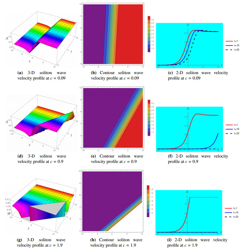
The study aims to explore the nonlinear Landau-Ginzburg-Higgs equation, which describes nonlinear waves with long-range and weak scattering interactions between tropical tropospheres and mid-latitude, as well as the exchange of mid-latitude Rossby and equatorial waves. We use the recently enhanced rising procedure to extract the important, applicable and further general solitary wave solutions to the formerly stated nonlinear wave model via the complex travelling wave transformation. Exact travelling wave solutions obtained include a singular wave, a periodic wave, bright, dark and kink-type wave peakon solutions using the generalized projective Riccati equation. The obtained findings are represented as trigonometric and hyperbolic functions. Graphical comparisons are provided for Landau-Ginzburg-Higgs equation model solutions, which are presented diagrammatically by adjusting the values of the embedded parameters in the Wolfram Mathematica program. The propagating behaviours of the obtained results display in 3-D, 2-D and contour visualization to investigate the impact of different involved parameters. The velocity of soliton has a stimulating effect on getting the desired aspects according to requirement. The sensitivity analysis is demonstrated for the designed dynamical structural system's wave profiles, where the soliton wave velocity and wave number parameters regulate the water wave singularity. This study shows that the method utilized is effective and may be used to find appropriate closed-form solitary solitons to a variety of nonlinear evolution equations (NLEEs).
Citation: Muhammad Imran Asjad, Sheikh Zain Majid, Waqas Ali Faridi, Sayed M. Eldin. Sensitive analysis of soliton solutions of nonlinear Landau-Ginzburg-Higgs equation with generalized projective Riccati method[J]. AIMS Mathematics, 2023, 8(5): 10210-10227. doi: 10.3934/math.2023517
The study aims to explore the nonlinear Landau-Ginzburg-Higgs equation, which describes nonlinear waves with long-range and weak scattering interactions between tropical tropospheres and mid-latitude, as well as the exchange of mid-latitude Rossby and equatorial waves. We use the recently enhanced rising procedure to extract the important, applicable and further general solitary wave solutions to the formerly stated nonlinear wave model via the complex travelling wave transformation. Exact travelling wave solutions obtained include a singular wave, a periodic wave, bright, dark and kink-type wave peakon solutions using the generalized projective Riccati equation. The obtained findings are represented as trigonometric and hyperbolic functions. Graphical comparisons are provided for Landau-Ginzburg-Higgs equation model solutions, which are presented diagrammatically by adjusting the values of the embedded parameters in the Wolfram Mathematica program. The propagating behaviours of the obtained results display in 3-D, 2-D and contour visualization to investigate the impact of different involved parameters. The velocity of soliton has a stimulating effect on getting the desired aspects according to requirement. The sensitivity analysis is demonstrated for the designed dynamical structural system's wave profiles, where the soliton wave velocity and wave number parameters regulate the water wave singularity. This study shows that the method utilized is effective and may be used to find appropriate closed-form solitary solitons to a variety of nonlinear evolution equations (NLEEs).

| [1] |
W. A. Faridi, M. I. Asjad, F. Jarad, Non-linear soliton solutions of perturbed Chen-Lee-Liu model by $\Phi^{6}-$ model expansion approach, Opt. Quant. Electron., 54 (2022), 664. https://doi.org/10.1007/s11082-022-04077-w doi: 10.1007/s11082-022-04077-w

|
| [2] |
Z. Q. Li, S. F. Tian, J. J. Yang, On the soliton resolution and the asymptotic stability of N-soliton solution for the Wadati-Konno-Ichikawa equation with finite density initial data in space-time solitonic regions, Adv. Math., 409 (2022), 108639. https://doi.org/10.1016/j.aim.2022.108639 doi: 10.1016/j.aim.2022.108639
|
| [3] |
S. Z. Majid, W. A. Faridi, M. I. Asjad, A. El-Rahman, S. M. Eldin, Explicit soliton structure formation for the Riemann Wave equation and a sensitive demonstration, Fractal Fract., 7 (2023), 102. https://doi.org/10.3390/fractalfract7020102 doi: 10.3390/fractalfract7020102
|
| [4] |
Z. Q. Li, S. F. Tian, J. J. Yang, Soliton resolution for the Wadati–Konno–Ichikawa equation with weighted Sobolev initial data, Ann. Henri Poincaré., 23 (2022), 2611–2655. https://doi.org/10.1007/s00023-021-01143-z doi: 10.1007/s00023-021-01143-z
|
| [5] |
L. L. Bu, F. Baronio, S. H. Chen, S. Trillo, Quadratic Peregrine solitons resonantly radiating without higher-order dispersion, Opt. Lett., 47 (2022), 2370–2373. https://doi.org/10.1364/OL.456187 doi: 10.1364/OL.456187
|
| [6] |
Z. Li, X. Y. Xie, C. J. Jin, Phase portraits and optical soliton solutions of coupled nonlinear Maccari systems describing the motion of solitary waves in fluid flow, Results Phy., 41 (2022), 105932. https://doi.org/10.1016/j.rinp.2022.105932 doi: 10.1016/j.rinp.2022.105932
|
| [7] |
Y. Shen, B. Tian, X. T. Gao, Bilinear auto-Bäcklund transformation, soliton and periodic-wave solutions for a (2+1)-dimensional generalized Kadomtsev–Petviashvili system in fluid mechanics and plasma physics, Chinese J. Phys., 77 (2022), 2698–2706. https://doi.org/10.1016/j.cjph.2021.11.025 doi: 10.1016/j.cjph.2021.11.025
|
| [8] |
K. K. Ali, C. Cattani, J. F. Gómez-Aguilar, D. Baleanu, M. S. Osman, Analytical and numerical study of the DNA dynamics arising in oscillator-chain of Peyrard-Bishop model, Chaos Soliton. Fract., 139 (2020), 110089. https://doi.org/10.1016/j.chaos.2020.110089 doi: 10.1016/j.chaos.2020.110089
|
| [9] |
M. S. Aktar, M. A. Akbar, M. S. Osman, Spatio-temporal dynamic solitary wave solutions and diffusion effects to the nonlinear diffusive predator-prey system and the diffusion-reaction equations, Chaos Soliton. Fract., 160 (2022), 112212. https://doi.org/10.1016/j.chaos.2022.112212 doi: 10.1016/j.chaos.2022.112212
|
| [10] |
O. A. Bruzzone, D. V. Perri, M. H. Easdale, Vegetation responses to variations in climate: A combined ordinary differential equation and sequential Monte Carlo estimation approach, Ecol. Inform., 73 (2022), 101913. https://doi.org/10.1016/j.ecoinf.2022.101913 doi: 10.1016/j.ecoinf.2022.101913
|
| [11] |
T. Y. Zhou, B. Tian, C. R. Zhang, S. H. Liu, Auto-Bäcklund transformations, bilinear forms, multiple-soliton, quasi-soliton and hybrid solutions of a (3+1)-dimensional modified Korteweg-de Vries-Zakharov-Kuznetsov equation in an electron-positron plasma, Eur. Phys. J. Plus, 137 (2022), 912. https://doi.org/10.1140/epjp/s13360-022-02950-x doi: 10.1140/epjp/s13360-022-02950-x
|
| [12] |
M. Alabedalhadi, Exact travelling wave solutions for nonlinear system of spatiotemporal fractional quantum mechanics equations, Alex. Eng. J., 61 (2022), 1033–1044. https://doi.org/10.1016/j.aej.2021.07.019 doi: 10.1016/j.aej.2021.07.019
|
| [13] |
L. Akinyemi, H. Rezazadeh, S. W. Yao, M. A. Akbar, M. M. Khater, A. Jhangeer, et al., Nonlinear dispersion in parabolic law medium and its optical solitons, Results Phy., 26 (2021), 104411. https://doi.org/10.1016/j.rinp.2021.104411 doi: 10.1016/j.rinp.2021.104411
|
| [14] |
L. Akinyemi, M. Şenol, H. Rezazadeh, H. Ahmad, H. Wang, Abundant optical soliton solutions for an integrable (2+1)-dimensional nonlinear conformable Schrödinger system, Results Phy., 25 (2021), 104177. https://doi.org/10.1016/j.rinp.2021.104177 doi: 10.1016/j.rinp.2021.104177
|
| [15] |
M. R. A. Fahim, P. R. Kundu, M. E. Islam, M. A. Akbar, M. S. Osman, Wave profile analysis of a couple of (3+1)-dimensional nonlinear evolution equations by sine-Gordon expansion approach, J. Ocean Eng. Sci., 7 (2022), 272–279. https://doi.org/10.1016/j.joes.2021.08.009 doi: 10.1016/j.joes.2021.08.009
|
| [16] |
Z. Q. Li, S. F. Tian, J. J. Yang, E. G. Fan, Soliton resolution for the complex short pulse equation with weighted Sobolev initial data in space-time solitonic regions, J. Differ. Equations, 329 (2022), 31–88. https://doi.org/10.1016/j.jde.2022.05.003 doi: 10.1016/j.jde.2022.05.003
|
| [17] |
S. Kumar, S. K. Dhiman, D. Baleanu, M. S. Osman, A. M. Wazwaz, Lie symmetries, closed-form solutions and various dynamical profiles of solitons for the variable coefficient (2+1)-dimensional KP equations, Symmetry, 14 (2022), 597. https://doi.org/10.3390/sym14030597 doi: 10.3390/sym14030597
|
| [18] |
A. Zafar, M. Shakeel, A. Ali, L. Akinyemi, H. Rezazadeh, Optical solitons of nonlinear complex Ginzburg–Landau equation via two modified expansion schemes, Opt. Quant. Electron., 54 (2022), 5. https://doi.org/10.1007/s11082-021-03393-x doi: 10.1007/s11082-021-03393-x
|
| [19] |
K. K. Ali, A. M. Wazwaz, M. S. Osman, Optical soliton solutions to the generalized nonautonomous nonlinear Schrödinger equations in optical fibers via the sine-Gordon expansion method, Optik, 208 (2020), 164132. https://doi.org/10.1007/s11082-021-03393-x doi: 10.1007/s11082-021-03393-x
|
| [20] |
R. Zhang, S. Bilige, T. Chaolu, Fractal solitons, arbitrary function solutions, exact periodic wave and breathers for a nonlinear partial differential equation by using bilinear neural network method, J. Syst. Sci. Complex., 34 (2021), 122–139. https://doi.org/10.1007/s11424-020-9392-5 doi: 10.1007/s11424-020-9392-5
|
| [21] |
M. Khater, A. Jhangeer, H. Rezazadeh, L. Akinyemi, M. A. Akbar, M. Inc, et al., New kinds of analytical solitary wave solutions for ionic currents on microtubules equation via two different techniques, Opt. Quant. Electron., 53 (2021), 609. https://doi.org/10.1007/s11082-021-03267-2 doi: 10.1007/s11082-021-03267-2
|
| [22] |
B. Karaman, The use of improved-F expansion method for the time-fractional Benjamin–Ono equation, Racsam. Rev. R. Acad. A., 115 (2021), 128. https://doi.org/10.1007/s13398-021-01072-w doi: 10.1007/s13398-021-01072-w
|
| [23] |
E. M. Zayed, K. A. Gepreel, R. M.Shohib, M. E. Alngar, Y. Yıldırım, Optical solitons for the perturbed Biswas-Milovic equation with Kudryashov's law of refractive index by the unified auxiliary equation method, Optik, 230 (2021), 166286. https://doi.org/10.1016/j.ijleo.2021.166286 doi: 10.1016/j.ijleo.2021.166286
|
| [24] |
H. F. Ismael, H. Bulut, H. M. Baskonus, Optical soliton solutions to the Fokas–Lenells equation via sine-Gordon expansion method and $(m+ ({G^{'}}/{G}))(m+({G^{'}}/{G}))$-expansion method, Pramana-J. Phys., 94 (2020), 35. https://doi.org/10.1007/s12043-019-1897-x doi: 10.1007/s12043-019-1897-x
|
| [25] | T. Abdulkadir Sulaiman, A. Yusuf, Dynamics of lump-periodic and breather waves solutions with variable coefficients in liquid with gas bubbles, Wave. Random Complex, in press. https://doi.org/10.1080/17455030.2021.1897708 |
| [26] |
F. S. Khodadad, S. M. Mirhosseini-Alizamini, B. Günay, L. Akinyemi, H. Rezazadeh, M. Inc, Abundant optical solitons to the Sasa-Satsuma higher-order nonlinear Schrödinger equation, Opt. Quant. Electron., 53 (2021), 702. https://doi.org/10.1007/s11082-021-03338-4 doi: 10.1007/s11082-021-03338-4
|
| [27] |
K. K. Ali, A. Yokus, A. R. Seadawy, R. Yilmazer, The ion sound and Langmuir waves dynamical system via computational modified generalized exponential rational function, Chaos Soliton. Fract., 161 (2022), 112381. https://doi.org/10.1016/j.chaos.2022.112381 doi: 10.1016/j.chaos.2022.112381
|
| [28] |
S. F. Tian, M. J. Xu, T. T. Zhang, A symmetry-preserving difference scheme and analytical solutions of a generalized higher-order beam equation, P. Roy. Soc. A-Math. Phy., 477 (2021), 20210455. https://doi.org/10.1098/rspa.2021.0455 doi: 10.1098/rspa.2021.0455
|
| [29] |
A. S. Rashed, S. M. Mabrouk, A. M. Wazwaz, Forward scattering for non-linear wave propagation in (3+1)-dimensional Jimbo-Miwa equation using singular manifold and group transformation methods, Wave. Random Complex, 32 (2022), 663–675. https://doi.org/10.1080/17455030.2020.1795303 doi: 10.1080/17455030.2020.1795303
|
| [30] |
S. Kumar, S. Rani, Symmetries of optimal system, various closed-form solutions and propagation of different wave profiles for the Boussinesq–Burgers system in ocean waves, Phys. Fluids, 34 (2022), 037109. https://doi.org/10.1063/5.0085927 doi: 10.1063/5.0085927
|
| [31] |
M. A. Abdulwahhab, Hamiltonian structure, optimal classification, optimal solutions and conservation laws of the classical Boussinesq–Burgers system, Partial Differential Equations in Applied Mathematics, 6 (2022), 100442. https://doi.org/10.1016/j.padiff.2022.100442 doi: 10.1016/j.padiff.2022.100442
|
| [32] |
C. C. Pan, L. L. Bu, S. H. Chen, W. X. Yang, D. Mihalache, P. Grelu, et al., General rogue wave solutions under SU (2) transformation in the vector Chen–Lee–Liu nonlinear Schrödinger equation, Physica D, 434 (2022), 133204. https://doi.org/10.1016/j.physd.2022.133204 doi: 10.1016/j.physd.2022.133204
|
| [33] |
D. S. Wang, H. Q. Zhang, Further improved F-expansion method and new exact solutions of the Konopelchenko-Dubrovsky equation, Chaos Soliton. Fract., 25 (2005), 601–610. https://doi.org/10.1016/j.chaos.2004.11.026 doi: 10.1016/j.chaos.2004.11.026
|
| [34] |
M. Alquran, T. A. Sulaiman, A. Yusuf, Kink-soliton, singular-kink-soliton and singular-periodic solutions for a new two-mode version of the Burger–Huxley model: applications in nerve fibers and liquid crystals, Opt. Quant. Electron., 53 (2021), 227. https://doi.org/10.1007/s11082-021-02883-2 doi: 10.1007/s11082-021-02883-2
|
| [35] |
M. A. Akbar, L. Akinyemi, S. W. Yao, A. Jhangeer, H. Rezazadeh, M. M. Khater, et al., Soliton solutions to the Boussinesq equation through sine-Gordon method and Kudryashov method, Results Phys., 25 (2021), 104228. https://doi.org/10.1016/j.rinp.2021.104228 doi: 10.1016/j.rinp.2021.104228
|
| [36] |
U. Asghar, W. A. Faridi, M. I. Asjad, S. M. Eldin, The enhancement of energy-carrying capacity in liquid with Gas Bubbles, in Terms of Solitons, Symmetry, 14 (2022), 2294. https://doi.org/10.3390/sym14112294 doi: 10.3390/sym14112294
|
| [37] |
W. A. Faridi, M. I. Asjad, S. M. Eldin, Exact fractional solution by Nucci's reduction approach and new analytical propagating optical soliton structures in Fiber-Optics, Fractal Fract., 6 (2022), 654. https://doi.org/10.3390/fractalfract6110654 doi: 10.3390/fractalfract6110654
|
| [38] |
S. Kumar, S. Malik, H. Rezazadeh, L. Akinyemi, The integrable Boussinesq equation and it's breather, lump and soliton solutions, Nonlinear Dynam., 107 (2022), 2703–2716. https://doi.org/10.1007/s11071-021-07076-w doi: 10.1007/s11071-021-07076-w
|
| [39] |
J. J. Yang, S. F. Tian, Z. Q. Li, Riemann–Hilbert problem for the focusing nonlinear Schrödinger equation with multiple high-order poles under nonzero boundary conditions, Physica D, 432 (2022), 133162. https://doi.org/10.1016/j.physd.2022.133162 doi: 10.1016/j.physd.2022.133162
|
| [40] |
S. T. Rizvi, A. R. Seadawy, U. Akram, New dispersive optical soliton for an nonlinear Schrödinger equation with Kudryashov law of refractive index along with P-test, Opt. Quant. Electron., 54 (2022), 1–23. https://doi.org/10.1007/s11082-022-03711-x doi: 10.1007/s11082-022-03711-x
|
| [41] |
M. E. Islam, M. A. Akbar, Stable wave solutions to the Landau-Ginzburg-Higgs equation and the modified equal width wave equation using the IBSEF method, Arab Journal of Basic and Applied Sciences, 27 (2020), 270–278. https://doi.org/10.1080/25765299.2020.1791466 doi: 10.1080/25765299.2020.1791466
|
| [42] |
A. Iftikhar, A. Ghafoor, T. Zubair, S. Firdous, S. T. Mohyud-Din, (G'/G, 1/G)-Expansion method for traveling wave solutions of (2+1) dimensional generalized KdV, Sin Gordon and Landau-Ginzburg-Higgs Equations, Sci. Res. Essays, 8 (2013), 1349–1359. https://doi.org/10.5897/SRE2013.5555 doi: 10.5897/SRE2013.5555
|
| [43] |
K. Ahmad, K. Bibi, M. S. Arif, K. Abodayeh, New exact solutions of Landau-Ginzburg-Higgs equation using power index method, J. Funct. Space, 2023 (2023), 4351698. https://doi.org/10.1155/2023/4351698 doi: 10.1155/2023/4351698
|
| [44] | M. R. Ali, M. A. Khattab, S. M. Mabrouk, Travelling wave solution for the Landau-Ginburg-Higgs model via the inverse scattering transformation method, Nonlinear Dynam., in press. https://doi.org/10.1007/s11071-022-08224-6 |
| [45] |
W. P. Hu, Z. C. Deng, S. M. Han, W. Fa, Multi-symplectic Runge-Kutta methods for Landau-Ginzburg-Higgs equation, Appl. Math. Mech., 30 (2009), 1027–1034. https://doi.org/10.1007/s10483-009-0809-x doi: 10.1007/s10483-009-0809-x
|
| [46] | C. Gomez, A. Salas, Exact solutions for the generalized shallow water wave equation by the general projective Riccati equations method, Bol. Mat., 13 (2006), 50–56. |
| [47] |
E. M. Zayed, K. A. Alurrfi, The generalized projective Riccati equations method and its applications for solving two nonlinear PDEs describing microtubules, Int. J. Phys. Sci., 10 (2015), 391–402. 10.5897/IJPS2015.4289 doi: 10.5897/IJPS2015.4289
|
| [48] | E. Yomba, General projective Riccati equations method and exact solutions for a class of nonlinear partial differential equations, IMA Preprint Series, 2004, 1–15. |


Figures(5)

Muhammad Imran Asjad, Sheikh Zain Majid, Waqas Ali Faridi, Sayed M. Eldin. Sensitive analysis of soliton solutions of nonlinear Landau-Ginzburg-Higgs equation with generalized projective Riccati method[J]. AIMS Mathematics, 2023, 8(5): 10210-10227. doi: 10.3934/math.2023517


 DownLoad: