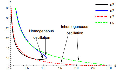
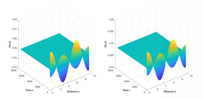
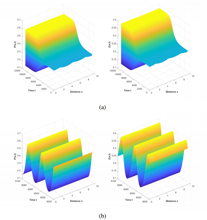
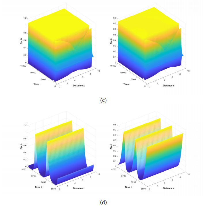
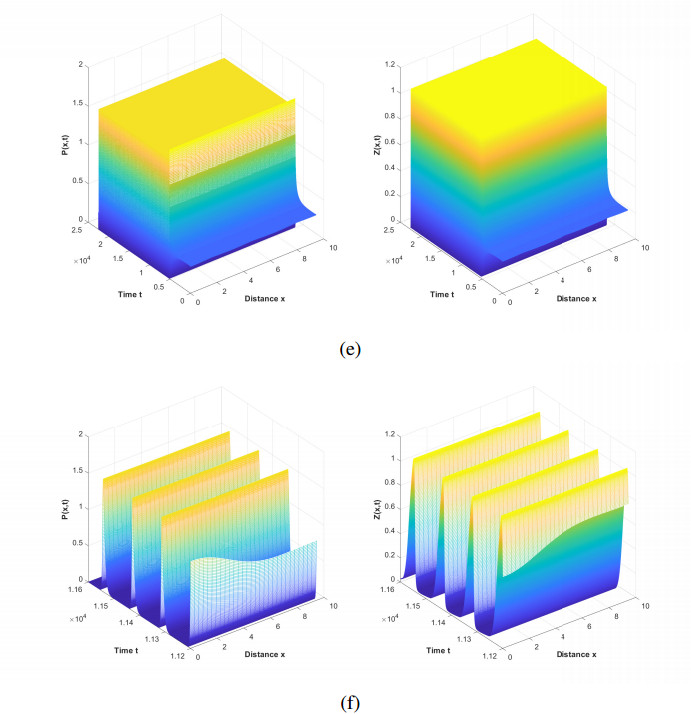
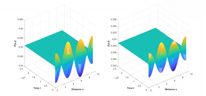
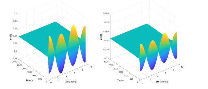
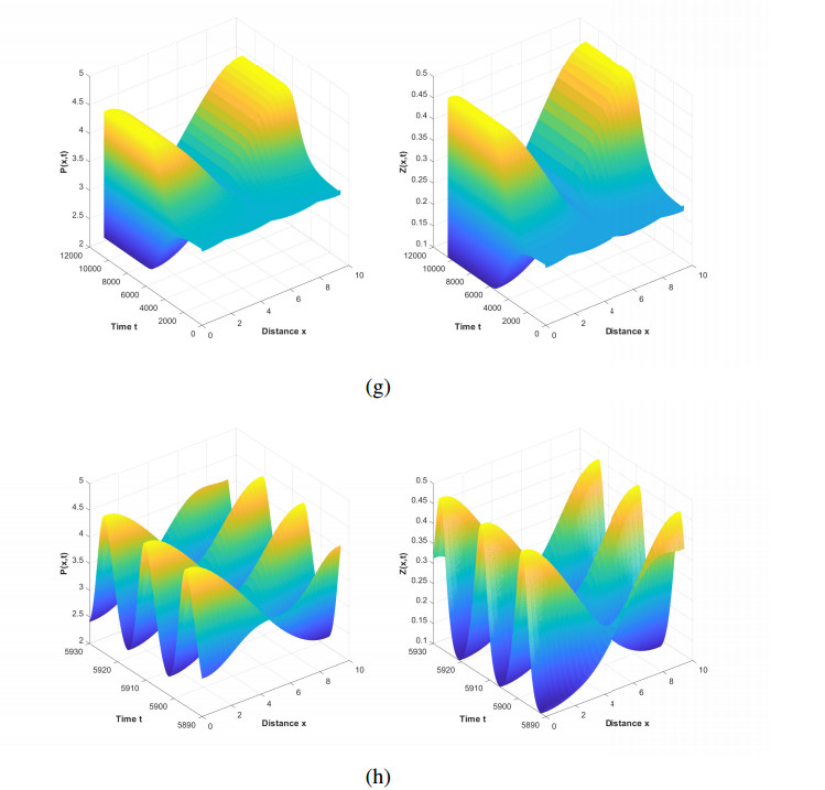
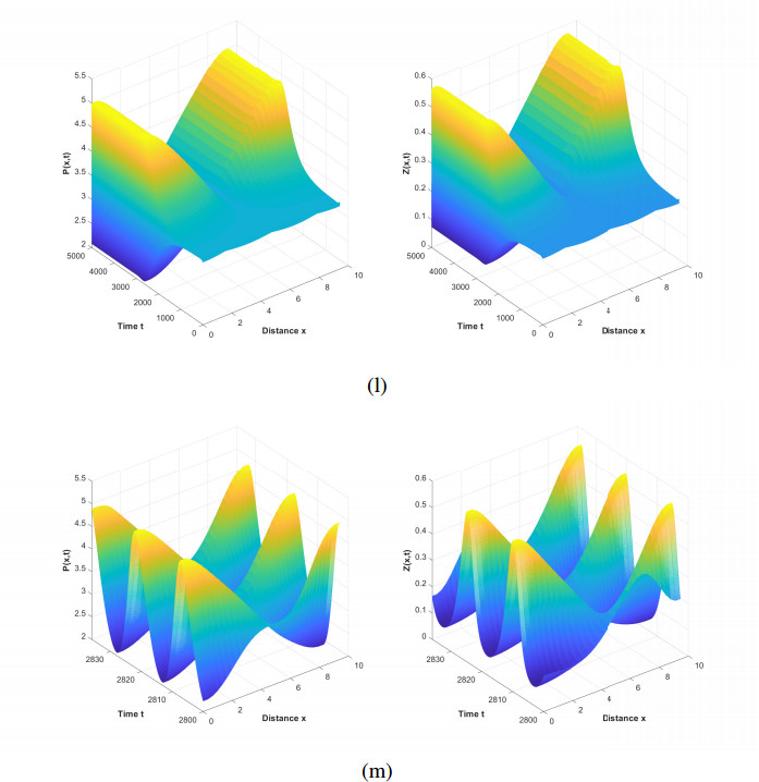
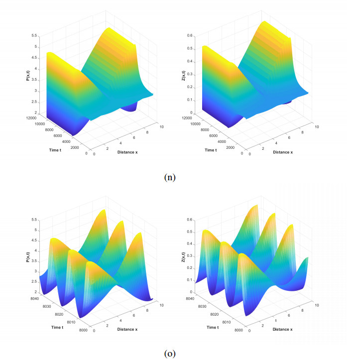
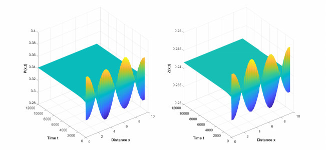
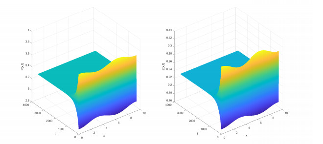
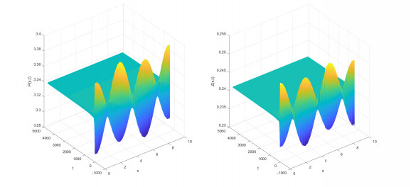
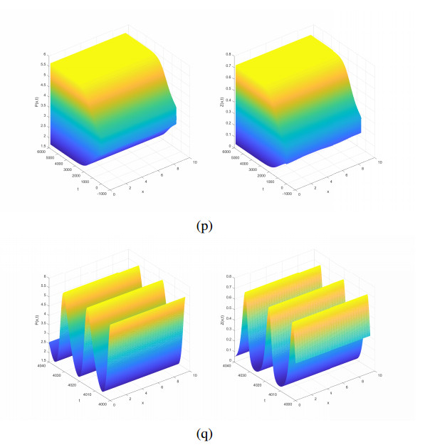
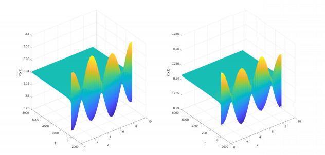
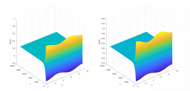
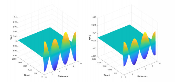
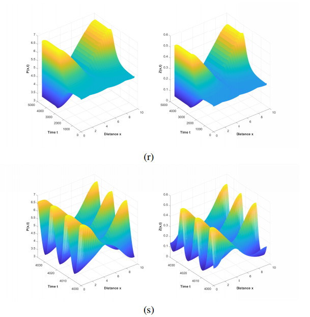
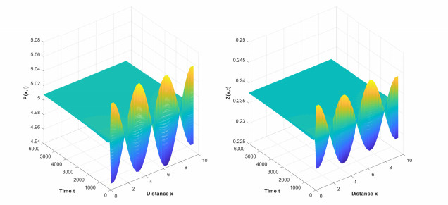
Since the distribution of plankton is always uneven, the nonlocal phytoplankton competition term indicates the spatial weighted mean of phytoplankton density, which is introduced into the plankton model with toxic substances effect to study the corresponding dynamic behavior. The stability of the positive equilibrium point and the existence of Hopf bifurcations are discussed by analysing the distribution of eigenvalues. The direction and stability of bifurcation periodic solution are researched based on an extended central manifold method and normal theory. Finally, spatially inhomogeneous oscillations are observed in the vicinity of the Hopf bifurcations. Through numerical simulation, we can observe that the system without nonlocal competition term only generates homogeneous periodic solution, and inhomogeneous periodic solution will produce only when both diffusion and nonlocal competition exist simultaneously. We can also see that when the toxin-producing rate of each phytoplankton is in an appropriate range, the system with nonlocal competition generates a stability switch with inhomogeneous periodic solution, when the value of time delay is in a certain interval, then Hopf bifurcations will appear, and with the increase of time delay, the quantity of plankton will eventually become stable.
Citation: Liye Wang, Wenlong Wang, Ruizhi Yang. Stability switch and Hopf bifurcations for a diffusive plankton system with nonlocal competition and toxic effect[J]. AIMS Mathematics, 2023, 8(4): 9716-9739. doi: 10.3934/math.2023490
Since the distribution of plankton is always uneven, the nonlocal phytoplankton competition term indicates the spatial weighted mean of phytoplankton density, which is introduced into the plankton model with toxic substances effect to study the corresponding dynamic behavior. The stability of the positive equilibrium point and the existence of Hopf bifurcations are discussed by analysing the distribution of eigenvalues. The direction and stability of bifurcation periodic solution are researched based on an extended central manifold method and normal theory. Finally, spatially inhomogeneous oscillations are observed in the vicinity of the Hopf bifurcations. Through numerical simulation, we can observe that the system without nonlocal competition term only generates homogeneous periodic solution, and inhomogeneous periodic solution will produce only when both diffusion and nonlocal competition exist simultaneously. We can also see that when the toxin-producing rate of each phytoplankton is in an appropriate range, the system with nonlocal competition generates a stability switch with inhomogeneous periodic solution, when the value of time delay is in a certain interval, then Hopf bifurcations will appear, and with the increase of time delay, the quantity of plankton will eventually become stable.

| [1] |
R. Pal, D. Basu, M. Banerjee, Modelling of phytoplankton allelopathy with Monod-Haldane-type functional response-A mathematical study, Biosystems, 95 (2009), 243–253. https://doi.org/10.1016/j.biosystems.2008.11.002 doi: 10.1016/j.biosystems.2008.11.002

|
| [2] |
S. Chakraborty, P. K. Tiwari, A. K. Misra, J. Chattopadhyay, Spatial dynamics of a nutrient-phytoplankton system with toxic effect on phytoplankton, Math. Biosci., 264 (2015), 94–100. https://doi.org/10.1016/j.mbs.2015.03.010 doi: 10.1016/j.mbs.2015.03.010
|
| [3] |
X. Y. Meng, Y. Q. Wu, Dynamical analysis of a fuzzy phytoplankton-zooplankton model with refuge, fishery protection and harvesting, J. Appl. Math. Comput., 63 (2020), 361–389. http://doi.org/10.1007/s12190-020-01321-y doi: 10.1007/s12190-020-01321-y
|
| [4] |
F. Zhang, J. Sun, W. Tian, Spatiotemporal pattern selection in a nontoxic-phytoplankton-toxic-phytoplankton-zooplankton model with toxin avoidance effects, Appl. Math. Comput., 423 (2022), 127007. https://doi.org/10.1016/j.amc.2022.127007 doi: 10.1016/j.amc.2022.127007
|
| [5] |
T. Zhang, W. Wang, Hopf bifurcation and bistability of a nutrient-phytoplankton-zooplankton model, Appl. Math. Model., 36 (2012), 6225–6235. https://doi.org/10.1016/j.apm.2012.02.012 doi: 10.1016/j.apm.2012.02.012
|
| [6] |
A. Mondal, S. Mondal, S. Mandal, Empirical dynamic model deciphers more information on the nutrient (N)-phytoplankton (P)-zooplankton (Z) dynamics of Hooghly-Matla estuary, Sundarban, India. Estuar. Coast. Shelf Sci., 265 (2022), 107711. https://doi.org/10.1016/j.ecss.2021.107711 doi: 10.1016/j.ecss.2021.107711
|
| [7] |
F. Zhang, W. Zhou, L. Yao, X. Wu, H. Zhang, Spatiotemporal patterns formed by a discrete Nutrient-Phytoplankton model with time delay, Complexity, 2020 (2020), 8541432. https://doi.org/10.1155/2020/8541432 doi: 10.1155/2020/8541432
|
| [8] |
K. Zhuang, Y. Li, B. Gong, Stability switches and Hopf bifurcation induced by nutrient recycling delay in a reaction-diffusion nutrient-phytoplankton model, Complexity, 2021 (2021), 7943788. https://doi.org/10.1155/2021/7943788 doi: 10.1155/2021/7943788
|
| [9] |
R. Yang, D. Jin, W. Wang, A diffusive predator-prey model with generalist predator and time delay, AIMS Mathematics, 7 (2022), 4574–4591. https://doi.org/10.3934/math.2022255 doi: 10.3934/math.2022255
|
| [10] |
R. Yang, X. Zhao, Y. An, Dynamical analysis of a delayed diffusive predator-prey model with additional food provided and anti-predator behavior, Mathematics, 10 (2022), 469. https://doi.org/10.3390/math10030469 doi: 10.3390/math10030469
|
| [11] |
R. Yang, Q. Song, Y. An, Spatiotemporal dynamics in a predator-prey model with functional response increasing in both predator and prey densities, Mathematics, 10 (2022), 17. https://doi.org/10.3390/math10010017 doi: 10.3390/math10010017
|
| [12] |
J. Chattopadhyay, R. R. Sarkar, A. E. Abdllaoui, A delay differential equation model on harmful algal blooms in the presence of toxic substances, Math. Med. Biol., 19 (2002), 137–161. https://doi.org/10.1093/imammb/19.2.137 doi: 10.1093/imammb/19.2.137
|
| [13] |
J. Zhao, J. Wei, Dynamics in a diffusive plankton system with delay and toxic substances effect, Nonlinear Anal. Real World Appl., 22 (2015), 66–83. https://doi.org/10.1016/j.nonrwa.2014.07.010 doi: 10.1016/j.nonrwa.2014.07.010
|
| [14] |
N. F. Britton, Aggregation and the competitive exclusion principle, J. Theor. Biol., 136 (1989), 57–66. https://doi.org/10.1016/S0022-5193(89)80189-4 doi: 10.1016/S0022-5193(89)80189-4
|
| [15] |
J. Furter, M. Grinfeld, Local vs. non-local interactions in population dynamics, J. Math. Biol., 27 (1989), 65–80. https://doi.org/10.1007/BF00276081 doi: 10.1007/BF00276081
|
| [16] |
D. Geng, W. Jiang, Y. Lou, H. Wang, Spatiotemporal patterns in a diffusive predator-prey system with nonlocal intraspecific prey competition, Stud. Appl. Math., 148 (2022), 396–432. https://doi.org/10.1111/sapm.12444 doi: 10.1111/sapm.12444
|
| [17] |
S. Pal, S. Petrovskii, S. Ghorai, M. Banerjee, Spatiotemporal pattern formation in 2D prey-predator system with nonlocal intraspecific competition, Commun. Nonlinear Sci. Numer. Simul., 93 (2021), 105478. https://doi.org/10.1016/j.cnsns.2020.105478 doi: 10.1016/j.cnsns.2020.105478
|
| [18] |
M. K. Pal, S. Poria, Effects of non-local competition on plankton-fish dynamics, Chaos, 31 (2021), 053108. https://doi.org/10.1063/5.0040844 doi: 10.1063/5.0040844
|
| [19] |
S. Wu, Y. Song, Stability and spatiotemporal dynamics in a diffusive predator-prey model with nonlocal prey competition, Nonlinear Anal. Real World Appl., 48 (2019), 12–39. https://doi.org/10.1016/j.nonrwa.2019.01.004 doi: 10.1016/j.nonrwa.2019.01.004
|
| [20] |
R. Yang, C. Nie, D. Jin, Spatiotemporal dynamics induced by nonlocal competition in a diffusive predator-prey system with habitat complexity, Nonlinear Dyn., 110 (2022), 879–900. https://doi.org/10.1007/s11071-022-07625-x doi: 10.1007/s11071-022-07625-x
|
| [21] |
R. Yang, F. Wang, D. Jin, Spatially inhomogeneous bifurcating periodic solutions induced by nonlocal competition in a predator-prey system with additional food, Math. Methods Appl. Sci., 45 (2022), 9967–9978. https://doi.org/10.1002/mma.8349 doi: 10.1002/mma.8349
|
| [22] |
S. Chen, J. Shi, Stability and Hopf bifurcation in a diffusive logistic population model with nonlocal delay effect, J. Differ. Equ., 253 (2012), 3440–3470. https://doi.org/10.1016/j.jde.2012.08.031 doi: 10.1016/j.jde.2012.08.031
|
| [23] | J. Wu, Theory and Applications of Partial Functional Differential Equations, New York: Springer, 1996. https://doi.org/10.1007/978-1-4612-4050-1 |
| [24] | B. D. Hassard, N. D. Kazarinoff, Y. H. Wan, Theory and Applications of Hopf Bifurcation, Cambridge: Cambridge University Press, 1981. http://doi.org/10.1090/conm/445 |
| [25] |
C. Xu, M. Liao, P. Li, Y. Guo, Z. Liu, Bifurcation properties for fractional order delayed BAM neural networks, Cognit. Comput., 13 (2021), 322–356. https://doi.org/10.1007/s12559-020-09782-w doi: 10.1007/s12559-020-09782-w
|
Figures(19)

Liye Wang, Wenlong Wang, Ruizhi Yang. Stability switch and Hopf bifurcations for a diffusive plankton system with nonlocal competition and toxic effect[J]. AIMS Mathematics, 2023, 8(4): 9716-9739. doi: 10.3934/math.2023490


 DownLoad: