Disaster decision-making with a mixing regret philosophy DDAS method in Fermatean fuzzy number

Aliya Fahmi; Rehan Ahmed; Muhammad Aslam; Thabet Abdeljawad; Aziz Khan; Aliya Fahmi; Rehan Ahmed; Muhammad Aslam; Thabet Abdeljawad; Aziz Khan

doi:10.3934/math.2023192

AIMS Mathematics

2023, Volume 8, Issue 2: 3860-3884. doi: 10.3934/math.2023192

Previous Article Next Article

Research article Special Issues

Disaster decision-making with a mixing regret philosophy DDAS method in Fermatean fuzzy number

1.
Department of Mathematics, Department of mathematics, University of Faisalabad, Faisalabad
2.
Department of Meteorology, COMSATS University, Islamabad, Pakistan
3.
Department of Mathematics, College of Sciences, Khalid University Abha, Saudi Arabia
4.
Department of Mathematics and Sciences, Prince Sultan University, P.O. Box 66833, 11586 Riyadh, Saudi Arabia
5.
Department of Medical Research, China Medical University, Taichung 40402, Taiwan

Received: 22 August 2022 Revised: 09 November 2022 Accepted: 10 November 2022 Published: 29 November 2022
MSC : 03B52, 03E72

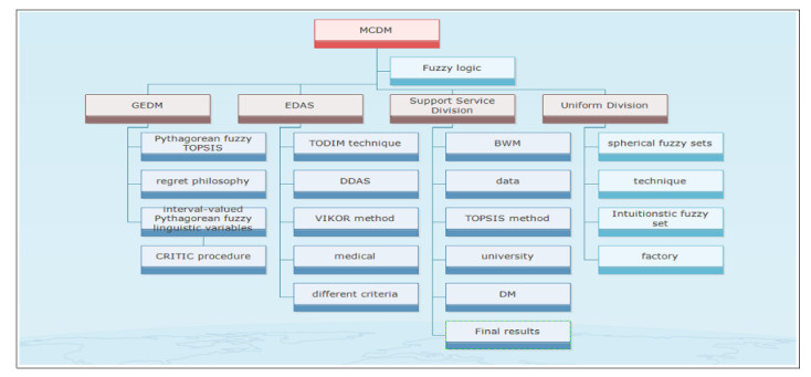
In this paper, the use of the Fermatean fuzzy number (FFN) in a significant research problem of disaster decision-making by defining operational laws and score function is demonstrated. Generally, decision control authorities need to brand suitable and sensible disaster decisions in the direct conceivable period as unfitting decisions may consequence in enormous financial dead and thoughtful communal costs. To certify that a disaster comeback can be made, professionally, we propose a new disaster decision-making (DDM) technique by the Fermatean fuzzy Schweizer-Sklar environment. First, the Fermatean fuzzy Schweizer-Sklar operators are employed by decision-makers to rapidly analyze their indefinite and vague assessment information on disaster choices. Then, the DDM technique based on the FFN is planned to identify highly devastating disaster choices and the best available choices. Finally, the proposed regret philosophy DDM technique is shown functional to choose the ideal retort explanation for a communal fitness disaster in Pakistan. The dominance and realism of the intended technique are further defensible through a relative study with additional DDM systems.

Keywords:

Citation: Aliya Fahmi, Rehan Ahmed, Muhammad Aslam, Thabet Abdeljawad, Aziz Khan. Disaster decision-making with a mixing regret philosophy DDAS method in Fermatean fuzzy number[J]. AIMS Mathematics, 2023, 8(2): 3860-3884. doi: 10.3934/math.2023192

Related Papers:

[1]	Hansaem Oh, Gwanghyun Jo . Physics-informed neural network for the heat equation under imperfect contact conditions and its error analysis. AIMS Mathematics, 2025, 10(4): 7920-7940. doi: 10.3934/math.2025364
[2]	Pengfei Zhu, Kai Liu . Numerical investigation of convergence in the $L^{\infty}$ norm for modified SGFEM applied to elliptic interface problems. AIMS Mathematics, 2024, 9(11): 31252-31273. doi: 10.3934/math.20241507
[3]	Hyun Geun Lee, Youngjin Hwang, Yunjae Nam, Sangkwon Kim, Junseok Kim . Benchmark problems for physics-informed neural networks: The Allen–Cahn equation. AIMS Mathematics, 2025, 10(3): 7319-7338. doi: 10.3934/math.2025335
[4]	Yu Xu, Youjun Deng, Dong Wei . Numerical solution of forward and inverse problems of heat conduction in multi-layered media. AIMS Mathematics, 2025, 10(3): 6144-6167. doi: 10.3934/math.2025280
[5]	Ruitao Liu, Wanshan Li . A new ADI-IIM scheme for solving two-dimensional wave equation with discontinuous coefficients. AIMS Mathematics, 2024, 9(11): 31180-31197. doi: 10.3934/math.20241503
[6]	Ahmed G. Salem, Turki D. Alharbi, Abdulaziz H. Alharbi, Anwar Ali Aldhafeeri . Impact of a spherical interface on a concentrical spherical droplet. AIMS Mathematics, 2024, 9(10): 28400-28420. doi: 10.3934/math.20241378
[7]	Dario Bambusi, Simone Paleari . A couple of BO equations as a normal form for the interface problem. AIMS Mathematics, 2024, 9(8): 23012-23026. doi: 10.3934/math.20241118
[8]	Min Wu, Jiali Zhou, Chaoyue Guan, Jing Niu . A numerical method using Legendre polynomials for solving two-point interface problems. AIMS Mathematics, 2025, 10(4): 7891-7905. doi: 10.3934/math.2025362
[9]	Xin Zhao, Xin Liu, Jian Li . Convergence analysis and error estimate of finite element method of a nonlinear fluid-structure interaction problem. AIMS Mathematics, 2020, 5(5): 5240-5260. doi: 10.3934/math.2020337
[10]	Maxime Krier, Julia Orlik . Solvability of a fluid-structure interaction problem with semigroup theory. AIMS Mathematics, 2023, 8(12): 29490-29516. doi: 10.3934/math.20231510

Abstract

1. Introduction

A class of problems that give rise of singular behavior are elliptic interface problems with imperfect contact ^[1], and it is featured by the implicit jump condition imposed on the imperfect contact interface, and the jumping quantity of the unknown is related to the flux across the interface. The elliptic interface problems with imperfect contact have been applied to model the Stefan problem of the solidification process and crystal growth, composite materials, multi-phase flows ^[2,3] and the problem of temperature discontinuity between the gas and cooling solid surface ^[4]. More examples include the heat conduction between materials of the different heat capacities and conductivities and interface diffusion processes ^[5,6], the temperature discontinuity between a gas and cooling solid surface ^[4], the conjugate heat transfer problem in thermodynamic processes between materials that are thermally coupled through non-adiabatic contacts ^[7], etc.

We consider the one-dimensional (1D) elliptic interface problem with imperfect contact

$\begin{equation} \begin{cases} & - ( \beta(x) u_{x})_x + c(x) u = f(x), \quad x\in (0, \alpha)\cup (\alpha, 1), \\ & u(0) = u_0, \quad u(1) = u_1, \end{cases} \end{equation}$

(1.1)

together with the following implicit jump conditions across the interface $\alpha$

$\begin{equation} \begin{cases} & [u] = u^{+} - u^{-} = \lambda \beta^{+} \nabla u^{+} \cdot \vec{n}, \\ & [\beta \frac{\partial u}{\partial \vec{n}}] = 0, \end{cases} \end{equation}$

(1.2)

where $0 < \alpha < 1$ , $\vec{n}$ is a unit normal to the interface pointing from $\Omega^{-}$ to $\Omega^{+}$ . $g^{\pm}$ denotes the right and left limits of the function $g$ at the point $\alpha$ , and $[g] = g^{+} - g^{-}$ . Without loss of generality, we assume that $\Omega$ is computational domain, and the interface $\alpha$ separates $\Omega$ into two sub-domains $\Omega^{-}$ and $\Omega^{+}$ .

The solution of the elliptic interface problems is often discontinuous due to discontinuous coefficients or singular sources across the interface. To recover the numerical accuracy near the interface, a variety of methods have been developed via enforcing the jump conditions (1.2) and (1.1) into numerical discretization such that accurate and robust numerical algorithms can be designed. Finite difference methods (FDMs) constitute a commonly used approach for elliptic interface problems. Since the publication of the original immersed interface method (IIM) ^[8], they have been applied to various problems, such as the Stokes flow with elastic boundaries or surface tension ^[9], incompressible flow based on the Navier-Stokes equations with singular source terms ^[10], and nonlinear problems in magneto-rheological fluids ^[11]. Many further developments and analysis in various aspects of the FDM for elliptic interface problems were carried out to improve the accuracy, stability or efficiency ^{[12,13,14,15,16,17,18,19]}. Many other elegant methods have been proposed in the past decade, including the ghost fluid method ^[20,21], finite volume method ^[7,22,23,24], the matched interface and boundary (MIB) method ^[25,26,27], etc. Finite element methods (FEMs) constitute another common practice to resolve the elliptic interface problems. With the help of body-fitted unstructured meshes, FEMs ^[28,29,30] have been developed for handling elliptic interfaces and irregular geometries. For interfaces with complex topologies, the construction of high quality body-fitted meshes could be difficult and time-consuming. This motivates the development of immersed FEMs based on non-body-fitted structured meshes ^{[31,32,33,34,35,36,37,38]}, etc. Nevertheless, most interface schemes in the literatures are designed to be of second-order accuracy.

The strategy for generating higher-order difference schemes can be roughly divided into two categories. (1) The first category is expanding the stencil and including more points in the schemes ^{[15,16,25,26,27,39,40,41,42]}. Advantages of this approaches is achieving high-order accuracy and using lower order jump conditions only. The obvious disadvantages of such approach is creating large matrix bandwidths and complicating the numerical treatment near the boundaries. Gibou and Fedkiw ^[16] introduced an $O(h^4)$ accurate finite difference discretization for the Laplace and heat equations on an irregular domain. Previous scholars ^[25,26,27] presented high-order MIB methods for solving elliptic equations with discontinuous coefficients and singular sources on Cartesian grids. This type of method is based on the use of fictitious points to achieve high-order accuracy. Zhong ^[40] presented a high-order IIM with general jump conditions by employing fictitious points to achieve high-order accuracy and using lower-order jump conditions only. Similar to the MIB approach, a wide stencil with more points are involved at irregular points. Feng and Zhao ^[42] introduced a new Cartesian grid FDM based on the fourth-order accurate MIB method. Colnago et al. ^[15] presented a high-order IIM for solving Poisson equations with discontinuous coefficients on Cartesian grids, it combines the FDM and ghost node strategy and requires only the ordinary jumps of the function. (2) The second category involves using the differential equation and the interface relations as additional identities ^[13,39,41]. The advantage of this approach is that the scheme is compact and minimal stencil is used. The disadvantage is that to maintain high-order accuracy, it requires the knowledge of jump conditions of high-order derivatives. Li and Ito ^[13] constructed a fourth-order IIM by computing high-order jump conditions involving mixed derivatives. Linnick and Fasel ^[39] presented a high-order IIM for simulating unsteady incompressible flow in an irregular domain. Instead of using analytical jump conditions, they compute the jump conditions for higher derivatives numerically. Angelova and Vulkov ^[41] presented high-order compact FDM for elliptic equations with intersecting interfaces by using the differential equation and the jump (interface) relations as additional identities, which can be differentiated to eliminate higher-order local truncation errors. For FEMs, the higher-order convergence crucially depends on how well the interface is resolved by the triangular mesh. In practice, subparametric, isoparametric or superparametric elements are usually employed to secure the optimal order of $p+1$ in the $L_2$ norm for a polynomial order of $p$ , for both continuous ^[33,43] and discontinuous Galerkin ^{[34,35,44,45,46]} FEMs. It is worth pointing out that most of the numerical methods in literatures are aimed at the elliptical interface problem with homogeneous jump conditions $([u] = 0, [\beta u_{\vec{n}}] = 0)$ or nonhomogeneous jump conditions where the jumps of the temperature as well as the conductive heat flux along the interface are known explicitly (say $[u] = g_1$ , $[\beta \partial u/ \partial \vec{n}] = g_2$ , with known $g_1$ and $g_2$ ). When the elliptic interface problem has an implicit jump condition as in (1.2), there are comparatively few numerical methods for solving such problems.

In this paper, we consider the 1D elliptic interface problems with imperfect contact, where the implicit jump condition is a setting for the interface and the jump of the primary variable is proportional to the normal flux across the interface. A class of high-order FDMs is constructed for the 1D elliptic interface for both the body-fitted and non-body-fitted mesh. For each case, the second-, third- and fourth-order approximations of the implicit jump condition are provided by using the original variables on both sides of the interface and a set of jump conditions and its high order derivatives. Numerical examples are presented to verify the performance of the scheme. The numerical results show that the presented schemes can reach the theoretical accuracy for solving the elliptic interface problems with imperfect contact.

The rest of this paper is organized as follows. In Section 2, we formulate the scheme for 1D elliptic equations with imperfect interfaces. Section 3 constructs the approximation of the normal derivative for the interface. Section 4 computes the primary variables $u^{+}$ and $u^{-}$ for the interface. Numerical examples are provided in Section 5 to demonstrate the accuracy and stability of the presented scheme. A concluding remark is given in Section 6.

2. High-order compact difference scheme

We assume that $\beta(x)$ in (1.1) is a piecewise smooth function with a jump at the interface $\alpha$ , and that $\beta(x)$ has upper and lower boundries:

$\begin{equation} 0 < \beta_{min} \leq \beta(x) \leq \beta_{max}, \end{equation}$

(2.1)

where $\beta_{min}$ and $\beta_{max}$ are two constants. The source term $f(x)$ is piecewise smooth.

Introduce a uniform grid $x_i = ih, i = 0, 1, \cdots, n$ with $h = \frac{1}{n}$ . The fourth-order compact difference scheme is constructed and three-point computational stencil for each point is adopted. For node $i$ , the three points in computational stencil are $\{x_{i-1}, x_i, x_{i+1}\}$ . Without loss of generality, assume the interface $\alpha$ is located in a grid interval, $x_k \leq \alpha \leq x_{k+1}$ . Because of the interface is located in the stencil, the points $k$ and $k+1$ are named as irregular points, and $i \ne k, k+1$ are name as regular points.

At a regular point $i$ , i.e., $i \ne k, k+1$ , for convenience, we briefly give the construction process of the fourth order compact difference scheme, for more detailed information one can refer to Ref.[47].

$\begin{equation} -\beta \delta^{2}_{x} u_i - \beta_{x} \delta_x u_i + c_{i} u_{i} + \tau = f_{i}, \end{equation}$

(2.2)

where

$\begin{equation*} \delta^{2}_x u_i = \frac{ u_{i+1} - 2 u_{i} + u_{i-1} }{h^2}, \quad \delta_{x} u_{i} = \frac{ u_{i+1} - u_{i-1} }{2h}, \end{equation*}$

and

$\begin{equation*} \tau = \beta_{x} \frac{h^2}{3!}\frac{\partial^3 u }{\partial x^3}\Big{|}_i + \beta \frac{h^2}{12} \frac{\partial^4 u}{x^4}\Big{|}_i + O(h^4). \end{equation*}$

Dropping the term $\tau$ in (2.2), it is the standard second-order central difference scheme. In order to get fourth-order scheme, we have to handle the high-order derivative terms $\frac{\partial^3 u }{\partial x^3}$ and $\frac{\partial^4 u}{\partial x^4}$ . According to the governing equation (1.1), there is

$\begin{equation} u_{xx} = \frac{1}{\beta} ( - \beta_x u_x + c u - f ). \end{equation}$

(2.3)

Taking the first and second derivatives to (2.3) respectively, we have

$\begin{equation} u_{xxx} = \phi_1 u_{xx} + \phi_2 u_{x} + \phi_3 u + \phi_4 f + \phi_5 f_x, \end{equation}$

(2.4)

and

$\begin{equation} u_{xxxx} = \psi_1 u_{xx} + \psi_2 u_{x} + \psi_3 u + \psi_4, \end{equation}$

(2.5)

where

$\begin{eqnarray*} & & \phi_1 = -\frac{\beta_x}{\beta}, \quad \phi_2 = \frac{\beta^2_x}{\beta^2} - \frac{\beta_{xx}}{\beta} + \frac{c}{\beta}, \quad \phi_3 = -\frac{c \beta_x}{\beta^2}, \quad \phi_4 = \frac{\beta_x}{\beta^2} , \quad \phi_5 = - \frac{1}{\beta}, \\ & & \psi_1 = \phi^2_1 + \phi_{1, x} + \phi_2, \quad \psi_2 = \phi_1 \phi_2 + \phi_{2, x} + \phi_3, \quad \psi_3 = \phi_1 \phi_3 + \phi_{3, x}, \\ & & \psi_4 = (\phi_1 \phi_4 + \phi_{4, x})f + (\phi_1 \phi_5 + \phi_4 + \phi_{5, x}) f_x + \phi_5 f_{xx}, \\ & & \phi_{1, x} = \frac{\beta^2_{x} - \beta \beta_{xx} }{\beta^2} , \quad \phi_{2, x} = 2 \frac{\beta_x}{\beta} \frac{\beta \beta_{xx} - \beta^2}{\beta^2} - \frac{ \beta \beta_{xxx} - \beta_x \beta_{xx} }{\beta^2} - \frac{c \beta_x}{\beta^2}, \\ & & \phi_{3, x} = \frac{c ( 2 \beta^2_{x} - \beta \beta_{xx} )}{\beta^3}, \quad \phi_{4, x} = \frac{ \beta \beta_{xx} - 2 \beta^2_{x} }{\beta^3}, \quad \phi_{5, x} = \frac{\beta_x}{\beta^2}. \end{eqnarray*}$

Substituting (2.4) and (2.5) into (2.2) and approximating the first- and second-derivatives with the central difference, we can get the fourth-order compact scheme:

$\begin{equation} A_i u_{i+1} + B_i u_{i} + C_{i} u_{i-1} = F_i + O(h^4), \end{equation}$

(2.6)

where

$\begin{eqnarray*} & & A_i = \frac{-\beta + \phi_1 \beta_x \frac{h^2}{6} + \psi_1 \beta \frac{h^2}{12} }{h^2} + \frac{ -\beta_x + \phi_2 \beta_x \frac{h^2}{6} + \psi_2 \beta \frac{h^2}{12} }{2h}, \\ & & B_i = 2 \frac{-\beta + \phi_1 \beta_x \frac{h^2}{6} + \psi_1 \beta \frac{h^2}{12} }{h^2} + ( c + \phi_3 \beta_x \frac{h^2}{6} + \psi_3 \beta \frac{h^2}{12} ), \\ & & C_i = \frac{-\beta + \phi_1 \beta_x \frac{h^2}{6} + \psi_1 \beta \frac{h^2}{12} }{h^2} - \frac{ -\beta_x + \phi_2 \beta_x \frac{h^2}{6} + \psi_2 \beta \frac{h^2}{12} }{2h}, \\ & & F_i = f_i - \beta_x \frac{h^2}{6} (\phi_4 f_i + \phi_5 f_{x, i}) - \beta \frac{h^2}{12} \psi_4. \end{eqnarray*}$

2.1. Interface fitted with mesh

When the interface is in contact with one of the mesh nodes, it is referred to as the body-fitted case. Without loss of generality, we assume that the interface is located the mesh node $k$ , as shown in Figure 1.

Figure 1. Interface fitted with body.

DownLoad: Full-Size Img PowerPoint

In this case, the irregular nodes are $k-1$ and $k+1$ , and the compact stencil of these two irregular nodes are shown in Figure {2}. Then, the high order compact scheme at these two irregular nodes can be given as

$\begin{equation} \bar{A}_{k-1} u_{k-2} + \bar{B}_{k-1} u_{k-1} + \bar{C}_{k-1} u^{-} = \bar{F}_{k-1}, \end{equation}$

(2.7)

and

$\begin{equation} \bar{A}_{k+1} u^{+} + \bar{B}_{k+1} u_{k+1} + \bar{C}_{k+1} u_{k+2} = \bar{F}_{k+1}. \end{equation}$

(2.8)

Apparently, there are two auxiliary qualities $u^{-}$ and $u^{+}$ in the schemes. To apply the above scheme, it is necessary to approximate the $u^{-}$ and $u^{+}$ with adequate accuracy. We prepare to use the interface jump connecting conditions and establish the linear systems with $u^{+}$ and $u^{-}$ as variables. The difficulty lies in the high-order discretization of the first-order derivatives $u^{+}_{x}$ and $u^{-}_{x}$ on both sides of the interface.

$\begin{equation} \begin{cases} [u] = \lambda \beta^{+} u^{+}_{x}, \\ [\beta u_{\vec{n}}] = 0. \end{cases} \end{equation}$

(2.9)

Figure 2. Irregular point stencil for interface-fitted mesh.

DownLoad: Full-Size Img PowerPoint

Expand the $u_{k+1}$ and $u_{k-1}$ at the interface $\alpha$ by using the Taylor series, it reads

$\begin{eqnarray} u_{k+1} & = & u^{+} + h \frac{\partial u}{\partial x}\Big{|}^{+} + \frac{ h^2}{2!} \frac{{\partial}^2 u}{\partial x^2}\Big{|}^{+} + \frac{ h^3}{3!} \frac{{\partial}^3 u}{\partial x^3}\Big{|}^{+} + \frac{ h^4}{4!} \frac{{\partial}^4 u}{\partial x^4}\Big{|}^{+} \\ &+& \frac{ h^5}{5!} \frac{{\partial}^5 u}{\partial x^5}\Big{|}^{+} + O( h^6), \end{eqnarray}$

(2.10)

and

$\begin{eqnarray} u_{k-1} & = & u^{-} - h \frac{\partial u}{\partial x}\Big|^{-} + \frac{ h^2}{2!} \frac{{\partial}^2 u}{\partial x^2}\Big|^{-} - \frac{ h^3}{3!} \frac{{\partial}^3 u}{\partial x^3}\Big|^{-} + \frac{ h^4}{4!} \frac{{\partial}^4 u}{\partial x^4}\Big|^{-} \\ &-& \frac{ h^5}{5!} \frac{{\partial}^5 u}{\partial x^5}\Big|^{-} + O( h^6). \end{eqnarray}$

(2.11)

Rewritting the above two formulas, we can get the representations of $\frac{\partial u}{\partial x}\Big{|}^{+}$ and $\frac{\partial u}{\partial x}\Big{|}^{-}$ as follows

$\begin{eqnarray} \frac{\partial u}{\partial x}\Big{|}^{+} & = & \frac{u_{k+1} - u^{+}}{h} - \frac{ h }{2!} \frac{{\partial}^2 u}{\partial x^2}\Big{|}^{+} - \frac{ h^2}{3!} \frac{{\partial}^3 u}{\partial x^3}\Big{|}^{+} - \frac{ h^3}{4!} \frac{{\partial}^4 u}{\partial x^4}\Big{|}^{+} \\ &-& \frac{ h^4}{5!} \frac{{\partial}^5 u}{\partial x^5}\Big{|}^{+} + O( h^5), \end{eqnarray}$

(2.12)

$\begin{eqnarray} \frac{\partial u}{\partial x}\Big{|}^{-} & = & \frac{u^{-} - u_{k-1} }{h} + \frac{ h }{2!} \frac{{\partial}^2 u}{\partial x^2}\Big{|}^{-} - \frac{ h^2}{3!} \frac{{\partial}^3 u}{\partial x^3}\Big{|}^{-} + \frac{ h^3}{4!} \frac{{\partial}^4 u}{\partial x^4}\Big{|}^{-} \\ &-& \frac{ h^4}{5!} \frac{{\partial}^5 u}{\partial x^5}\Big{|}^{-} + O( h^5). \end{eqnarray}$

(2.13)

According to the governing equation, we have

$\begin{equation} u^{+}_{xx} = \frac{1}{\beta^{+}} ( - \beta^{+}_x u^{+}_x + c^{+} u^{+} - f^{+} ), \quad u^{-}_{xx} = \frac{1}{\beta^{-}} ( - \beta^{-}_x u^{-}_x + c^{-} u^{-} - f^{-} ). \end{equation}$

(2.14)

Keeping the first two terms on the right-hand side of (2.12) and substituting (2.14) into (2.12), the second-order accurate approximate scheme of $\frac{\partial u}{\partial x}\Big{|}^{+}$ can be given as

$\begin{equation} \frac{\partial u}{\partial x}\Big{|}^{+} = \rho_{r, 1} u^{+} + \rho_{r, 2} u_{k+1} + \rho_{r, 3} + O(h^2), \end{equation}$

(2.15)

where

$\begin{eqnarray*} \rho_{r, 1} = -(\frac{1}{h} + \frac{h}{2}\frac{c^{+}}{\beta^{+}})\Big{/}D_r , \quad \rho_{r, 2} = \frac{1}{h} \Big{/}D_r , \quad \rho_{r, 3} = \frac{h}{2}\frac{f^{+}}{\beta^{+}}\Big{/}D_r, \quad D_r = (1-\frac{h}{2}\frac{\beta^{+}_{x}}{\beta^{+}}). \end{eqnarray*}$

To obtain the higher-order approximate of $\frac{\partial u}{\partial x}\Big{|}^{+}$ , it is necessary to handle the third- and fourth-order derivatives in (2.12). From (2.4) and (2.5), the expressions of $u^{+}_{xxx}$ and $u^{+}_{xxxx}$ can be given as

$\begin{equation} u^{+}_{xxx} = \Phi^{+}_1 u^{+}_{x} + \Phi^{+}_2 u^{+} + \Phi^{+}_3, \end{equation}$

(2.16)

and

$\begin{equation} u^{+}_{xxxx} = \Psi^{+}_1 u^{+}_{x} + \Psi^{+}_2 u^{+} + \Psi^{+}_3, \end{equation}$

(2.17)

where

$\begin{eqnarray*} & & \Phi^{+}_1 = - \frac{\beta^{+}_x}{\beta^{+}} \phi^{+}_1 + \phi^{+}_2, \quad \Phi^{+}_2 = \frac{c^{+}}{\beta^{+}} \phi^{+}_1 + \phi^{+}_3, \quad \Phi^{+}_3 = (-\frac{c^{+}}{\beta^{+}}\phi^{+}_1 + \phi^{+}_4) f^{+} + \phi^{+}_5 f^{+}_x, \\ & & \Psi^{+}_1 = - \frac{\beta^{+}_x}{\beta^{+}} \psi^{+}_1 + \psi^{+}_2, \quad \Psi^{+}_2 = \frac{c^{+}}{\beta^{+}} \psi^{+}_1 + \psi^{+}_3, \quad \Psi^{+}_3 = \frac{f^{+}}{\beta^{+}}\psi^{+}_1 + \psi^{+}_4. \end{eqnarray*}$

Keeping the first three terms on the right-hand side of (2.12), we establish the third-order accurate approximate of $\frac{\partial u}{\partial x}\Big{|}^{+}$ as follows:

$\begin{equation} \frac{\partial u}{\partial x}\Big{|}^{+} = \bar{\rho}_{r, 1} u^{+} + \bar{\rho}_{r, 2} u_{k+1} + \bar{\rho}_{r, 3} + O(h^3), \end{equation}$

(2.18)

where

$\begin{eqnarray*} \bar{\rho}_{r, 1} & = & -\left(\frac{1}{h} + \frac{h}{2} \frac{c^{+}}{\beta^{+}} + \frac{h^2}{6}\Phi^{+}_2 \right)\big{/}\bar{D}_r, \quad \bar{\rho}_{r, 2} = \frac{1}{h}\big{/} \bar{D}_r , \\ \bar{\rho}_{r, 3} & = & \left(\frac{h}{2}\frac{f^{+}}{\beta^{+}} - \frac{h^2}{6} \Phi^{+}_3 \right)\big{/}\bar{D}_r, \quad \bar{D}_r = 1 - \frac{h}{2} \frac{\beta^{+}_x}{\beta^{+}} + \frac{h^2}{6} \Phi^{+}_1. \end{eqnarray*}$

Further, the fourth-order approximate of $\frac{\partial u}{\partial x}\Big{|}^{+}$ can be given as

$\begin{equation} \frac{\partial u}{\partial x}\Big{|}^{+} = \bar{\bar{\rho}}_{r, 1} u^{+} + \bar{\bar{\rho}}_{r, 2} u_{k+1} + \bar{\bar{\rho}}_{r, 3} + O(h^4), \end{equation}$

(2.19)

where

$\begin{eqnarray*} \bar{\bar{\rho}}_{r, 1} & = & - \left(\frac{1}{h} + \frac{h}{2} \frac{c^{+}}{\beta^{+}} + \frac{h^2}{6} \Phi^{+}_2 + \frac{h^3}{24}\Psi^{+}_2 \right) \big{/} \bar{\bar{D}}_r, \quad \bar{\bar{\rho}}_{r, 2} = \frac{1}{h} \big{/} \bar{\bar{D}}_r , \\ \bar{\bar{\rho}}_{r, 3} & = & \left(\frac{h}{2}\frac{f^{+}}{\beta^{+}} + \frac{h^2}{6} \Phi^{+}_3 + \frac{h^3}{24} \Psi^{+}_3 \right)\big{/} \bar{\bar{D}}_r, \quad \bar{\bar{D}}_r = 1 - \frac{h}{2}\frac{\beta^{+}_x}{\beta^{+}} - \frac{h^2}{6} \Phi^{+}_1 + \frac{h^3}{24} \Psi^{+}_1. \end{eqnarray*}$

Similarly, the second-, third- and fourth-order approximation of $\frac{\partial u}{\partial x}\Big{|}^{-}$ can be given as

$\begin{equation} \frac{\partial u}{\partial x}\Big{|}^{-} = \rho_{l, 1} u^{-} + \rho_{l, 2} u_{k-1} + \rho_{l, 3} + O(h^2), \end{equation}$

(2.20)

$\begin{equation} \frac{\partial u}{\partial x}\Big{|}^{-} = \bar{\rho}_{l, 1} u^{-} + \bar{\rho}_{l, 2} u_{k-1} + \bar{\rho}_{l, 3} + O(h^3), \end{equation}$

(2.21)

$\begin{equation} \frac{\partial u}{\partial x}\Big{|}^{-} = \bar{\bar{\rho}}_{l, 1} u^{-} + \bar{\bar{\rho}}_{l, 2} u_{k-1} + \bar{\bar{\rho}}_{l, 3} + O(h^4), \end{equation}$

(2.22)

where

$\begin{eqnarray*} \rho_{l, 1} & = & (\frac{1}{h} + \frac{h}{2} \frac{c^{-}}{\beta^{-}} ) \Big{/} D_l, \quad \rho_{l, 2} = -\frac{1}{h} \Big{/} D_l, \quad \rho_{l, 3} = -\frac{h}{2}\frac{f^{-}}{\beta^{-}}\Big{/} D_l, \quad D_l = 1 + \frac{h}{2} \frac{\beta^{-}_x}{\beta^{-}} , \\ \bar{\rho}_{l, 1} & = & \left(\frac{1}{h} + \frac{h}{2} \frac{c^{-}}{\beta^{-}} - \frac{h^2}{6} \Phi^{-}_2 \right) \big{/} \bar{D}_l, \quad \bar{\rho}_{l, 2} = -\frac{1}{h} \big{/} \bar{D}_l, \\ \bar{\rho}_{l, 3} & = & \left( -\frac{h}{2}\frac{f^{-}}{\beta^{-}} - \frac{h^2}{6} \Phi^{-}_3 \right) \big{/} \bar{D}_l, \quad \bar{D}_l = 1 + \frac{h}{2} \frac{\beta^{-}_x}{\beta^{-}} + \frac{h^2}{6} \Phi^{-}_1 , \\ \bar{\bar{\rho}}_{l, 1} & = & \left(\frac{1}{h} + \frac{h}{2} \frac{c^{-}}{\beta^{-}} - \frac{h^2}{6} \Phi^{-}_2 + \frac{h^3}{24} \Psi^{-}_2 \right) \big{/} \bar{\bar{D}}_l, \quad \bar{\bar{\rho}}_{l, 2} = -\frac{1}{h} \big{/} \bar{\bar{D}}_l, \\ \bar{\bar{\rho}}_{l, 3} & = & \left(-\frac{h}{2}\frac{f^{-}}{\beta^{-}} + \frac{h^2}{6} \Phi^{-}_3 + \frac{h^3}{24} \Psi^{-}_3 \right) \big{/} \bar{\bar{D}}_l , \quad \bar{\bar{D}}_l = 1 + \frac{h}{2} \frac{\beta^{-}_x}{\beta^{-}} - \frac{h^2}{6} \Phi^{-}_1 + \frac{h^3}{24} \Psi^{-}_1. \end{eqnarray*}$

2.2. Interface unfitted with mesh

When the interface is located within one of the computational mesh, it appears as shown in . The irregular nodes are $k$ and $k+1$ , and the construction of the higher order scheme is more complicated. Owing to the interface arbitrarily cutting through the computational mesh, the computational mesh of these irregular nodes is nonuniform, as shown in Figure 4.

Figure 3. Interface unfitted with a body.

DownLoad: Full-Size Img PowerPoint

Figure 4. Nonuniform mesh.

DownLoad: Full-Size Img PowerPoint

We assume the function $u(x)$ is smooth enough, expand the $u(x_{i+1}), u(x_{i-1})$ at point $x_i$ by Taylor series

$\begin{eqnarray} u_{i+1} & = & u_{i} + h_f \frac{\partial u}{\partial x}\Big{|}_{i} + \frac{ h^2_f}{2!} \frac{{\partial}^2 u}{\partial x^2}\Big{|}_{i} + \frac{ h^3_f}{3!} \frac{{\partial}^3 u}{\partial x^3}\Big{|}_{i} + \frac{ h^4_f}{4!} \frac{{\partial}^4 u}{\partial x^4}\Big{|}_{i} \\ &+& \frac{h^5_f}{5!} \frac{{\partial}^5 u}{\partial x^5}\Big{|}_{i} + O(h^6_f), \end{eqnarray}$

(2.23)

and

$\begin{eqnarray} u_{i-1} & = & u_{i} - h_b \frac{\partial u}{\partial x}\Big|_{i} + \frac{ h^2_b}{2!} \frac{{\partial}^2 u}{\partial x^2}\Big|_{i} - \frac{ h^3_b}{3!} \frac{{\partial}^3 u}{\partial x^3}\Big|_{i} + \frac{ h^4_b}{4!} \frac{{\partial}^4 u}{\partial x^4}\Big|_{i} \\ &-& \frac{h^5_b}{5!} \frac{{\partial}^5 u}{\partial x^5}\Big|_{i} + O(h^6_b). \end{eqnarray}$

(2.24)

From (2.23) and (2.24), we can obtain

$\begin{eqnarray} \frac{{\partial}^2 u}{\partial x^2}\Big|_{i} & = & 2 \frac{ h_b u_{i+1} + h_f u_{i-1} -( h_f + h_b) u_i }{h_f h_b (h_f + h_b)} - \frac{h_f - h_b}{3} \frac{{\partial}^3 u}{\partial x^3}\Big|_{i} - \frac{1}{12} \frac{h^3_f + h^3_b }{h_f + h_b} \frac{{\partial}^4 u}{\partial x^4}\Big|_{i} \\ &-& \frac{1}{60}(h^2_f + h^2_b)(h_f + h_b) \frac{{\partial}^5 u}{\partial x^5}\Big|_{i} + O(\frac{ h^5_f + h^5_b }{h_f + h_b}), \end{eqnarray}$

(2.25)

and

$\begin{eqnarray} \frac{{\partial} u}{\partial x}\Big|_{i} & = & \frac{ h^2_b u_{i+1} - h^2_f u_{i-1} + (h^2_f - h^2_b) u_i }{h^2_b h_f + h^2_f h_b} - \frac{ h_f h_b}{6} \frac{{\partial}^3 u}{\partial x^3}\Big|_{i} - \frac{h_f h_b (h_f - h_b) }{24} \frac{{\partial}^4 u}{\partial x^4}\Big|_{i} \\ &+& O(\frac{ (h^3_f + h^3_b)h_f h_b }{ h_f + h_b }). \end{eqnarray}$

(2.26)

Define the difference operators

$\begin{equation} \delta_{x} u_i = \frac{ h^2_b u_{i+1} - h^2_f u_{i-1} + (h^2_f - h^2_b) u_i }{h^2_b h_f + h^2_f h_b}, \end{equation}$

(2.27)

$\begin{equation} \delta^2_{x} u_i = 2 \frac{ h_b u_{i+1} + h_f u_{i-1} -( h_f + h_b) u_i }{h_f h_b (h_f + h_b)}. \end{equation}$

(2.28)

Equations (2.25) and (2.26) can be rewritten as

$\begin{eqnarray} \frac{{\partial}^2 u}{\partial x^2}\Big|_{i} & = & \delta^2_{x} u_i - \frac{h_f - h_b}{3} \frac{{\partial}^3 u}{\partial x^3}\Big|_{i} - \frac{1}{12} \frac{h^3_f + h^3_b }{h_f + h_b} \frac{{\partial}^4 u}{\partial x^4}\Big|_{i} \\ &-& \frac{1}{60}(h^2_f + h^2_b)(h_f + h_b) \frac{{\partial}^5 u}{\partial x^5}\Big|_{i} + O(\frac{ h^5_f + h^5_b }{h_f + h_b}), \end{eqnarray}$

(2.29)

and

$\begin{eqnarray} \frac{{\partial} u}{\partial x}\Big|_{i} = \delta_{x} u_i - \frac{ h_f h_b}{6} \frac{{\partial}^3 u}{\partial x^3}\Big|_{i} - \frac{h_f h_b (h_f - h_b) }{24} \frac{{\partial}^4 u}{\partial x^4}\Big|_{i} + O(\frac{ (h^3_f + h^3_b)h_f h_b }{ h_f + h_b }). \end{eqnarray}$

(2.30)

Substituting Eqs (2.29) and (2.30) into the governing equation (1.1), we can get the difference scheme for the elliptic interface equation

$\begin{equation} - \beta \delta^2_{x} u_i - \beta_{x} \delta_{x} u_i + k_i u_i + \tau = f_i, \end{equation}$

(2.31)

where

$\begin{eqnarray} \tau = Q_1 \frac{{\partial}^3 u}{\partial x^3}\Big|_{i} + Q_2 \frac{{\partial}^4 u}{\partial x^4}\Big|_{i} + Q_3 \frac{{\partial}^5 u}{\partial x^5}\Big|_{i} + O(h^4), \end{eqnarray}$

(2.32)

and

$\begin{eqnarray*} Q_1 & = & \beta \frac{h_f - h_b}{3} - \beta_x \frac{h_f h_b}{6}, \quad Q_2 = \beta \frac{1}{12} \frac{h^3_f + h^3_b}{h_f + h_b} - \beta_x \frac{h_f h_b (h_f - h_b)}{24} , \\ Q_3 & = & \beta \frac{1}{60}(h^2_f + h^2_b)(h_f + h_b). \end{eqnarray*}$

To obtain the higher-order accuracy discrete scheme, it is necessary to handle the third- and fourth-order derivatives of the term $\tau$ . Substituting (2.4) and (2.5) into (2.31) and rearranging it, we have

$\begin{equation} \mathcal{A}_i \delta^2_{x} u_i + \mathcal{B} \delta_x u_i + \mathcal{C}_i u_i = \mathcal{F}_i + O((h^2_f + h^2_b)(h_f + h_b)), \end{equation}$

(2.33)

where

$\begin{eqnarray*} \mathcal{A}_i = -\beta + Q_1 \phi_1 + Q_2 \psi_1, \quad \mathcal{B}_i = -\beta_x + Q_1 \phi_2 + Q_2 \psi_2, \\ \mathcal{C}_i = c_i + Q_1 \phi_3 + Q_2 \psi_3, \quad \mathcal{F}_i = f_i - Q_1 (\phi_4 f_i + \phi_5 f_{x, i}) - Q_2 \psi_4. \end{eqnarray*}$

For the irregular points $k$ and $k+1$ , we use the interface $\alpha$ as one of the points in the compact stencil as shown in . Thus, the 3-point compact stencil for nodes $k$ and $k+1$ are $k-1, k, \alpha^{-}$ and $\alpha^{+}, k+1, k+2$ , respectively. From the above analysis, the difference operators for the first- and second-order derivatives for nodes $k$ and $k+1$ are respectively as follows

$\begin{equation} \delta_{x} u_k = \frac{ h^2_b u^{-} - h^2_f u_{k-1} + (h^2_f - h^2_b) u_k }{h^2_b h_f + h^2_f h_b}, \quad \delta^2_{x} u_k = 2 \frac{ h_b u^{-} + h_f u_{k-1} -( h_f + h_b) u_k }{h_f h_b (h_f + h_b)}, \end{equation}$

(2.34)

Figure 5. Stencil of interface unfitted with a body.

DownLoad: Full-Size Img PowerPoint

and

$\begin{equation} \delta_{x} u_{k+1} = \frac{ h^2_b u_{k+2} - h^2_f u^{+} + (h^2_f - h^2_b) u_{k+1} }{h^2_b h_f + h^2_f h_b}, \quad \delta^2_{x} u_{k+1} = 2 \frac{ h_b u_{k+2} + h_f u^{+} -( h_f + h_b) u_{k+1} }{h_f h_b (h_f + h_b)}. \end{equation}$

(2.35)

Substituting (2.34) and (2.35) into (2.33), we can get the higher-order compact scheme for the irregular point $k$ :

$\begin{equation} \bar{A}_k u_{k-1} + \bar{B}_k u_{k} + \bar{C}_k u^{-} = \bar{F}_k + O((h^2_f + h^2_b)(h_f + h_b)), \end{equation}$

(2.36)

where

$\begin{eqnarray*} &&\bar{A}_k = \frac{2}{h_b (h_f + h_b) } \mathcal{A}_k - \frac{h^2_f }{h^2_b h_f + h^2_f h_b } \mathcal{B}_k , \quad \bar{B}_k = - \frac{2}{h_f h_b } \mathcal{A}_k + \frac{ h^2_f - h^2_b }{h^2_b h_f + h^2_f h_b } \mathcal{B}_k + \mathcal{C}_k, \\ &&\bar{C}_k = \frac{2}{h_f (h_f + h_b)} \mathcal{A}_k + \frac{h^2_b}{h^2_b h_f + h^2_f h_b} \mathcal{B}_k , \quad \bar{F}_k = \mathcal{F}_k. \end{eqnarray*}$

Similarly, the higher-order compact scheme for the irregular point $k+1$ is as follows:

$\begin{equation} \bar{A}_{k+1} u^{+} + \bar{B}_{k+1} u_{k+1} + \bar{C}_{k+1} u_{k+2} = \bar{F}_{k+1}+ O((h^2_f + h^2_b)(h_f + h_b)), \end{equation}$

(2.37)

where

$\begin{eqnarray*} &&\bar{A}_{k+1} = \frac{2}{h_b (h_f + h_b)} \mathcal{A}_{k+1} - \frac{h^2_f}{h^2_b h_f + h^2_f h_b} \mathcal{B}_{k+1} , \\ &&\bar{B}_{k+1} = - \frac{2}{h_f h_b} \mathcal{A}_{k+1} + \frac{h^2_f - h^2_b}{h^2_b h_f + h^2_f h_b} \mathcal{B}_{k+1} + \mathcal{C}_{k+1}, \\ &&\bar{C}_{k+1} = \frac{2}{h_f (h_f + h_b)} \mathcal{A}_{k+1} + \frac{h^2_b}{h^2_b h_f + h^2_f h_b} \mathcal{B}_{k+1} , \quad \bar{F}_{k+1} = \mathcal{F}_{k+1}. \end{eqnarray*}$

From the above analysis, we have constructed the higher-order compact scheme at regular points and irregular points. It should be noted that there are two auxiliary unknown quantities $u^{+}$ and $u^{-}$ in the scheme for the irregular points $k$ and $k+1$ . Therefore, we have to find a way to deal with the interface connection conditions, so as to obtain a high-precision approximation for the auxiliary unknowns $u^{+}$ and $u^{-}$ on both sides of the interface.

3. Approximation of the normal derivative on the interface

The first order derivative on both sides of the interface, $\frac{\partial u}{\partial x}\Big{|}^{+}$ and $\frac{\partial u}{\partial x}\Big{|}^{-}$ , can respectively be given as

$\begin{eqnarray} \frac{\partial u}{\partial x}\Big{|}^{+} & = & \frac{u_{k+1} - u^{+}}{h_{r1}} - \frac{ h_{r1} }{2!} \frac{{\partial}^2 u}{\partial x^2}\Big{|}^{+} - \frac{ h^2_{r1}}{3!} \frac{{\partial}^3 u}{\partial x^3}\Big{|}^{+} - \frac{ h^3_{r1}}{4!} \frac{{\partial}^4 u}{\partial x^4}\Big{|}^{+} \\ &-& \frac{ h^4_{r1}}{5!} \frac{{\partial}^5 u}{\partial x^5}\Big{|}^{+} + O( h^5_r), \end{eqnarray}$

(3.1)

and

$\begin{eqnarray} \frac{\partial u}{\partial x}\Big{|}^{-} & = & \frac{u^{-} - u_{k} }{h_{l1}} + \frac{ h_{l1} }{2!} \frac{{\partial}^2 u}{\partial x^2}\Big{|}^{-} - \frac{ h^2_{l1}}{3!} \frac{{\partial}^3 u}{\partial x^3}\Big{|}^{-} + \frac{ h^3_{l1}}{4!} \frac{{\partial}^4 u}{\partial x^4}\Big{|}^{-} \\ &-& \frac{ h^4_{l1}}{5!} \frac{{\partial}^5 u}{\partial x^5}\Big{|}^{-} + O( h^5_l), \end{eqnarray}$

(3.2)

where $h_{l1} = \alpha - x_k$ , $h_{r1} = x_{k+1} - \alpha$ , $h_{l2} = h_{l1} + h$ and $h_{r2} = h_{r1} + h$ , as shown in Figure 6.

Figure 6. Interface and the irregular nodes.

DownLoad: Full-Size Img PowerPoint

Further, the second-order derivative on both sides of the interface, $\frac{\partial^2 u}{\partial x^2}\Big{|}^{+}$ and $\frac{\partial^2 u}{\partial x^2}\Big{|}^{-}$ , can respectively be given as

$\begin{eqnarray} \frac{\partial^2 u}{\partial x^2}\Big{|}^{+} & = & \frac{-2}{h_{r1} h_{r2} h} \left(h_{r2}u_{k+1} - h_{r1} u_{k+2} - h u^{+} \right) - \frac{ h_{r1} + h_{r2}}{3} \frac{{\partial}^3 u}{\partial x^3}\Big{|}^{+} \\ &-& \frac{h^2_{r1} + h_{r1}h_{r2} + h^{2}_{r2}}{12} \frac{{\partial}^4 u}{\partial x^4}\Big{|}^{+} + O( h^3_{r1}+ h^{2}_{r2} h_{r1} + h^{2}_{r1} h_{r2} + h^{3}_{r2}), \end{eqnarray}$

(3.3)

and

$\begin{eqnarray} \frac{\partial^2 u}{\partial x^2}\Big{|}^{-} & = & \frac{-2}{h_{l1} h_{l2} h} \left( h_{l2} u_{k} - h_{l1} u_{k-1} - h u^{-} \right) + \frac{ h_{l1} + h_{l2}}{3} \frac{{\partial}^3 u}{\partial x^3}\Big{|}^{-} \\ &-& \frac{h^2_{l1} + h_{l1}h_{l2} + h^{2}_{l2}}{12} \frac{{\partial}^4 u}{\partial x^4}\Big{|}^{-} + O( h^3_{l1}+h^{2}_{l2}h_{l1}+h^{2}_{l1}h_{l2}+h^{3}_{l2}). \end{eqnarray}$

(3.4)

Substituting (3.3) and (3.4) into (3.1) and (3.2) respectively, we can get

$\begin{eqnarray} \frac{\partial u}{\partial x}\Big{|}^{+} & = & \big\{ -(\frac{1}{h_{r1}} + \frac{1}{h_{r2}}) u^{+} + ( \frac{1}{h_{r1}} + \frac{1}{h}) u_{k+1} - \frac{h_{r1}}{h_{r2} h} u_{k+2} \big\} + \frac{ h_{r1}h_{r2}}{3!} \frac{{\partial}^3 u}{\partial x^3}\Big{|}^{+} \\ &+& \frac{h^2_{r1}h_{r2} + h^{2}_{r2} h_{r1}}{4!} \frac{{\partial}^4 u}{\partial x^4}\Big{|}^{+} + O( h^3_{r1}+h^{2}_{r2}h_{r1}+h^{2}_{r1}h_{r2}+h^{3}_{r2}), \end{eqnarray}$

(3.5)

and

$\begin{eqnarray} \frac{\partial u}{\partial x}\Big{|}^{-} & = & \big\{ (\frac{1}{h_{l1}} + \frac{1}{h_{l2}}) u^{-} - (\frac{1}{h_{l1}} + \frac{1}{h}) u_{k} + \frac{h_{l1}}{h_{l2} h} u_{k-1} \big\} + \frac{ h_{l1}h_{l2}}{3!} \frac{{\partial}^3 u}{\partial x^3}\Big{|}^{+} \\ &-& \frac{h^2_{l1}h_{l2} + h^{2}_{l2} h_{l1}}{4!} \frac{{\partial}^4 u}{\partial x^4}\Big{|}^{+} + O( h^3_{l1}+h^{2}_{l2}h_{l1}+h^{2}_{l1}h_{l2}+h^{3}_{l2}). \end{eqnarray}$

(3.6)

3.1. Second-order scheme

Keep the first term in (3.6) and (3.5) and discard the other terms. We can get the approximation of the first order derivative on both sides of the interface with second-order accuracy:

$\begin{equation} u^{-}_{x} = \rho_{l, 1} u^{-} + \rho_{l, 2} u_{k} + \rho_{l, 3}u_{k-1} + O(h^2), \end{equation}$

(3.7)

and

$\begin{equation} u^{+}_{x} = \rho_{r, 1} u^{+} + \rho_{r, 2} u^{k+1} + \rho_{r, 3}u_{k+2} + O(h^2), \end{equation}$

(3.8)

where

$\begin{eqnarray*} \rho_{l, 1} = \frac{1}{h_{l1}} + \frac{1}{h_{l2}} , \quad \rho_{l, 2} = - (\frac{1}{h_{l1}} + \frac{1}{h}), \quad \rho_{l, 3} = \frac{h_{l1}}{h h_{l2}}, \\ \rho_{r, 1} = -(\frac{1}{h_{r1}} + \frac{1}{h_{r2}}), \quad \rho_{r, 2} = \frac{1}{h_{r1}} + \frac{1}{h}, \quad \rho_{r, 3} = -\frac{h_{r1}}{h h_{r2}}. \end{eqnarray*}$

3.2. Third-order scheme

Keeping the first two terms in (3.6) and (3.5) and discarding the other terms, and according to the (2.16), we can get the approximation of the first derivative with third order accuracy

$\begin{equation} u^{-}_{x} = \bar{\rho}_{l, 1} u^{-} + \bar{\rho}_{l, 2} u_{k} + \bar{\rho}_{l, 3} u_{k-1} + \bar{\rho}_{l, 4} + O(h^3), \end{equation}$

(3.9)

and

$\begin{equation} u^{+}_{x} = \bar{\rho}_{r, 1} u^{+} + \bar{\rho}_{r, 2} u_{k+1} + \bar{\rho}_{r, 3} u_{k+2} + \bar{\rho}_{r, 4} + O(h^3), \end{equation}$

(3.10)

where

$\begin{eqnarray*} & & \bar{\rho}_{l, 1} = \left(\rho_{1, 1} + \frac{h_{l1} h_{l2}}{6} \Phi^{-}_2 \right) \big/\bar{D}_l, \quad \bar{\rho}_{l, 2} = \rho_{1, 2} \big/\bar{D}_l , \quad \bar{\rho}_{l, 3} = \rho_{1, 3}\big/\bar{D}_l, \\ & & \bar{\rho}_{l, 4} = \frac{h_{l1} h_{l2}}{6} \Phi^{-}_3 \big/\bar{D}_l , \quad \bar{D}_l = 1 - \frac{h_{l1} h_{l2}}{6} \Phi^{-}_1 , \\ & & \bar{\rho}_{r, 1} = \left(\rho_{r, 1} + \frac{h_{r1} h_{r2}}{6} \Phi^{+}_2 \right) \big/\bar{D}_r, \quad \bar{\rho}_{r, 2} = \rho_{r, 2}\big/ \bar{D}_r , \quad \bar{\rho}_{r, 3} = \rho_{r, 3}\big/\bar{D}_r , \\ & & \bar{\rho}_{l, 4} = \frac{h_{r1} h_{r2}}{6} \Phi^{+}_3 \big/\bar{D}_r, \quad \bar{D}_r = 1 - \frac{h_{r1} h_{r2}}{6} \Phi^{+}_1. \end{eqnarray*}$

3.3. Fourth order scheme

Following the same manner as in the above subsection, we can get the approximation of the first derivative with fourth-order accuracy

$\begin{equation} u^{-}_{x} = \bar{\bar{\rho}}_{l, 1} u^{-} + \bar{\bar{\rho}}_{l, 2} u_{k} + \bar{\bar{\rho}}_{l, 3} u_{k-1} + \bar{\bar{\rho}}_{l, 4} + O(h^4), \end{equation}$

(3.11)

and

$\begin{equation} u^{+}_{x} = \bar{\bar{\rho}}_{r, 1} u^{+} + \bar{\bar{\rho}}_{r, 2} u_{k+1} + \bar{\bar{\rho}}_{r, 3} u_{k+2} + \bar{\bar{\rho}}_{r, 4}+ O(h^4), \end{equation}$

(3.12)

where

$\begin{eqnarray*} & & \bar{\bar{\rho}}_{l, 1} = \left( \rho_{l, 1} + \frac{h_{l1} h_{l2}}{6} \Phi^{-}_2 + \frac{h^{2}_{l2} h_{l1} + h^{2}_{l1} h_{l2}}{24} \Psi^{-}_2 \right)\big/\bar{\bar{D}}_l, \quad \bar{\bar{\rho}}_{l, 2} = \rho_{l, 2} \big/\bar{\bar{D}}_l, \\ & & \bar{\bar{\rho}}_{l, 3} = \rho_{l, 3} \big/\bar{\bar{D}}_l, \quad \bar{\bar{\rho}}_{l, 4} = \left( \frac{h_{l1} h_{l2}}{6} \Phi^{-}_3 + \frac{h^{2}_{l2} h_{l1} + h^{2}_{l1} h_{l2}}{24} \Psi^{-}_3 \right)\big/ \bar{\bar{D}}_l, \\ & & \bar{\bar{\rho}}_{r, 1} = \left( \rho_{r, 1} - \frac{h_{l1} h_{l2}}{6} \Phi^{-}_1 - \frac{h^{2}_{l2} h_{l1} + h^{2}_{l1} h_{l2}}{24} \Psi^{-}_1 \right)\big/\bar{\bar{D}}_r, \quad \bar{\bar{\rho}}_{r, 2} = \rho_{r, 2} \big/\bar{\bar{D}}_r , \\ & & \bar{\bar{\rho}}_{r, 3} = \rho_{r, 3} \big/\bar{\bar{D}}_r, \quad \bar{\bar{\rho}}_{r, 4} = \left( \frac{h_{r1} h_{r2}}{6} \Phi^{+}_3 - \frac{h^{2}_{r2} h_{r1} + h^{2}_{r1} h_{r2}}{24} \Psi^{+}_3 \right)\big/\bar{\bar{D}}_r, \\ & & \bar{\bar{D}}_l = 1 - \frac{h_{l1} h_{l2}}{6} \Phi^{-}_1 - \frac{h^{2}_{r2} h_{r1} + h^{2}_{r1} h_{r2}}{24} \Psi^{+}_1 , \\ & & \bar{\bar{D}}_r = 1 - \frac{h_{r1} h_{r2}}{6} \Phi^{+}_1 - \frac{h^{2}_{r2} h_{r1} + h^{2}_{r1} h_{r2}}{24} \Psi^{+}_1 . \end{eqnarray*}$

4. Compute $u^{+}$ and $u^{-}$ on the interface

The implicit connecting condition on the interface is given as

$\begin{equation} \begin{cases} [u] = \lambda \beta^{-} u^{-}_{x}, \\ \beta^{+}u^{+}_{x} = \beta^{-} u^{-}_{x}. \end{cases} \end{equation}$

(4.1)

For the interface fitted mesh, the approximation of the first-order derivative on both sides of the interface can respectively be written as

$\begin{eqnarray} & & {\frac{\partial u}{\partial x}}\big{|}^{-} = \rho_{l, 1} u^{-} + \rho_{l, 2} u_{k-1} + \rho_{l, 3} + O(h^{m}_l), \end{eqnarray}$

(4.2)

$\begin{eqnarray} & & {\frac{\partial u}{\partial x}}\big{|}^{+} = \rho_{r, 1} u^{+} + \rho_{r, 2} u_{k+1} + \rho_{r, 3} + O(h^{m}_r). \end{eqnarray}$

(4.3)

Discarding the terms $O(h^{m}_l)$ and $O(h^{m}_r)$ in (4.2) and (4.3), and substituting them into (4.1), the discrete format of the implicit connecting condition on the interface can be given as

$\begin{equation*} \label{jumpcond3} \begin{cases} u^{+} - u^{-} = \lambda \beta^{-} (\rho_{l, 1} u^{-} + \rho_{l, 2} u_{k-1} + \rho_{l, 3}) , \\ \beta^{+}(\rho_{r, 1} u^{+} + \rho_{r, 2} u_{k+1} + \rho_{r, 3}) = \beta^{-} (\rho_{l, 1} u^{-} + \rho_{l, 2} u_{k-1} + \rho_{l, 3}) . \end{cases} \end{equation*}$

For brevity, rearrange the above equation and establish linear equations with $u^{+}$ and $u^{-}$ as variables as follows:

$\begin{equation*} \begin{cases} a_{11} u^{+} - a_{12} u^{-} = b_{1}, \\ a_{21} u^{+} + a_{22} u^{-} = b_{2}, \end{cases} \end{equation*}$

where

$\begin{eqnarray*} && a_{11} = 1, \quad a_{12} = 1 + \lambda {\beta}^{-} \rho_{l, 1}, \quad a_{21} = {\beta}^{+} \rho_{r, 1}, \quad a_{22} = -{\beta}^{-} \rho_{l, 1}. \\ && b_1 = \lambda {\beta}^{-} (\rho_{l, 2} u_{k-1} + \rho_{l, 3} ), \\ && b_2 = {\beta}^{-} (\rho_{l, 2} u_{k-1} + \rho_{l, 3} ) - {\beta}^{+} (\rho_{r, 2} u_{k+1} + \rho_{r, 3}). \end{eqnarray*}$

Solving the above linear system, we can get the approximate of each of the unknowns $u^{+}$ and $u^{-}$ on both sides of the interface with $m$ -th order accuracy:

$\begin{eqnarray} u^{+} & = & \tau^{+}_1 u_{k-1} + \tau^{+}_2 u_{k+1} + \tau^{+}_3, \end{eqnarray}$

(4.4)

$\begin{eqnarray} u^{-} & = & \tau^{-}_1 u_{k-1} + \tau^{-}_2 u_{k+1} + \tau^{-}_3, \end{eqnarray}$

(4.5)

where

$\begin{eqnarray*} &&\tau^{+}_{1} = \frac{ (a_{22} \lambda + a_{12})\beta^{-}\rho_{l, 2} }{a_{11}a_{22} + a_{12}a_{21}}, \quad \tau^{+}_{2} = -\frac{ a_{12} \beta^{+} \rho_{r, 2} }{a_{11}a_{22} + a_{12}a_{21}}, \\ &&\tau^{+}_{3} = \frac{ (a_{22} \lambda + a_{12})\beta^{-}\rho_{l, 3} - a_{12} \beta^{+} \rho_{r, 3} }{a_{11}a_{22} + a_{12}a_{21}} , \\ &&\tau^{-}_{1} = \frac{ (a_{11} - a_{21} \lambda)\beta^{-}\rho_{l, 2} }{a_{11}a_{22} + a_{12}a_{21}}, \quad \tau^{-}_{2} = -\frac{ a_{11} \beta^{+}\rho_{r, 2} }{a_{11}a_{22} + a_{12}a_{21}}, \\ &&\tau^{-}_{3} = \frac{ (a_{11} - a_{21} \lambda)\beta^{-}\rho_{l, 3} - a_{11} \beta^{+} \rho_{r, 3} }{a_{11}a_{22} + a_{12}a_{21}}. \end{eqnarray*}$

For the interface-cut mesh, the approximation of the first-order derivative on both sides of the interface can be written as

$\begin{eqnarray} & & {\frac{\partial u}{\partial x}}\big{|}^{-} = \rho_{l, 1} u^{-} + \rho_{l, 2} u_{k} + \rho_{l, 3} u_{k-1} + \rho_{l, 4} + O(h^{m}_l), \end{eqnarray}$

(4.6)

$\begin{eqnarray} & & {\frac{\partial u}{\partial x}}\big{|}^{+} = \rho_{r, 1} u^{+} + \rho_{r, 2} u_{k+1} + \rho_{r, 3}u_{k+2} + \rho_{r, 4} + O(h^{m}_r). \end{eqnarray}$

(4.7)

In a similar manner as above, the approximate of each of the unknowns $u^{+}$ and $u^{-}$ on both sides of the interface with $m$ -th-order accuracy is given as

$\begin{eqnarray} u^{+} & = & \tau^{+}_1 u_{k-1} + \tau^{+}_2 u_{k} + \tau^{+}_3 u_{k+1} + \tau^{+}_4 u_{k+2} + \tau^{+}_5, \end{eqnarray}$

(4.8)

$\begin{eqnarray} u^{-} & = & \tau^{-}_1 u_{k-1} + \tau^{-}_2 u_{k} + \tau^{-}_3 u_{k+1} + \tau^{-}_4 u_{k+2} + \tau^{-}_5, \end{eqnarray}$

(4.9)

where

$\begin{eqnarray*} &&\tau^{+}_{1} = \frac{ (a_{22} \lambda + a_{12})\beta^{-}\rho_{l, 3} }{a_{11}a_{22} + a_{12}a_{21}}, \quad \tau^{+}_{2} = \frac{ (a_{22} \lambda + a_{12})\beta^{-}\rho_{l, 2} }{a_{11}a_{22} + a_{12}a_{21}}, \quad \tau^{+}_{3} = \frac{ - a_{12} \beta^{+}\rho_{r, 2} }{a_{11}a_{22} + a_{12}a_{21}}, \\ &&\tau^{+}_{4} = \frac{ - a_{12} \beta^{+}\rho_{r, 3} }{a_{11}a_{22} + a_{12}a_{21}}, \quad \tau^{+}_{5} = \frac{ a_{22} \lambda \beta^{-} \rho_{l, 4} + a_{12} ( \beta^{-} \rho_{l, 4} - \beta^{+} \rho_{r, 4} ) }{a_{11}a_{22} + a_{12}a_{21}}, \\ &&\tau^{-}_{1} = \frac{ (a_{11} - a_{21} \lambda)\beta^{-}\rho_{l, 3} }{a_{11}a_{22} + a_{12}a_{21}}, \quad \tau^{-}_{2} = \frac{ (a_{11} - a_{21} \lambda)\beta^{-}\rho_{l, 2} }{a_{11}a_{22} + a_{12}a_{21}}, \quad \tau^{-}_{3} = \frac{ - a_{11} \beta^{+} \rho_{r, 2} }{a_{11}a_{22} + a_{12}a_{21}}, \\ &&\tau^{-}_{4} = \frac{ - a_{11} \beta^{+} \rho_{r, 3} }{a_{11}a_{22} + a_{12}a_{21}}, \quad \tau^{-}_{5} = \frac{ a_{11}( \beta^{-}\rho_{l, 4} - \beta^{+}\rho_{r, 4}) - a_{21} \lambda \beta^{-}\rho_{l, 4} }{a_{11}a_{22} + a_{12}a_{21}}. \end{eqnarray*}$

and

$\begin{eqnarray*} && a_{11} = 1, \quad a_{12} = 1 + \lambda {\beta}^{-} \rho_{l, 1}, \quad a_{21} = {\beta}^{+} \rho_{r, 1}, \quad a_{22} = -{\beta}^{-} \rho_{l, 1}. \\ && b_1 = \lambda {\beta}^{-} (\rho_{l, 2} u_{k} + \rho_{l, 3} u_{k-1} + \rho_{l, 4} ), \\ && b_2 = {\beta}^{-} (\rho_{l, 2} u_{k} + \rho_{l, 3} u_{k-1} + \rho_{l, 4} ) - {\beta}^{+} (\rho_{r, 2} u_{k+1} + \rho_{r, 3}u_{k+2} + \rho_{r, 4}). \end{eqnarray*}$

5. Discrete system

From the above sections, we establish the fourth-order compact finite-difference scheme for non-irregular mesh nodes:

$\begin{equation} A_i u_{i-1} + B_{i} u_i + C_{i} u_{i+1} = F_{i}, \end{equation}$

(5.1)

for

$\begin{equation*} i \neq \begin{cases} \{k-1, k+1 \}, \quad \quad {\rm{for\; body-fitted\; mesh, }} \\ \{k, k+1\}, \qquad \qquad{\rm{for \;non-body-fitted\; mesh}}. \end{cases} \end{equation*}$

In the interface-fitted mesh case, the higher-order compact schemes at the irregular mesh nodes $k-1$ and $k+1$ are given as (2.7) and (2.8), respectively. Eliminating the auxiliary qualities $u^{+}$ and $u^{-}$ by substituting the formulas (4.4) and (4.5) into (2.7) and (2.8). The schemes for the irregular mesh nodes are given as

$\begin{equation} A_{k-1} u_{k-2} + B_{k-1} u_{k-1} + C_{k-1} u_{k+1} = F_{k-1}, \end{equation}$

(5.2)

and

$\begin{equation} A_{k+1} u_{k-1} + B_{k+1} u_{k+1} + C_{k+1} u_{k+2} = F_{k+1}, \end{equation}$

(5.3)

where

$\begin{eqnarray*} & & A_{k-1} = \bar{A}_{k-1} , \quad B_{k-1} = \bar{B}_{k-1} + \bar{C}_{k-1} \tau^{-}_1, \quad C_{k-1} = \bar{C}_{k-1} \tau^{-}_2, \\ & & A_{k+1} = \bar{A}_{k+1} \tau^{+}_1 , \quad B_{k+1} = \bar{B}_{k+1} + \bar{A}_{k+1} \tau^{+}_2 , \quad C_{k+1} = \bar{C}_{k+1}, \\ & & F_{k-1} = \bar{F}_{k-1} - \bar{C}_{k-1} \tau^{-}_3, \quad F_{k+1} = \bar{F}_{k+1} - \bar{A}_{k+1} \tau^{+}_3 . \end{eqnarray*}$

Similarly, in the non-body-fitted case, the higher-order compact schemes at the irregular mesh nodes $k$ and $k+1$ are respectively given as (2.36) and (2.37). Substitute the formulas (4.8) and (4.9) into (2.36) and (2.37) to eliminate the auxiliary qualities $u^{+}$ and $u^{-}$ . The higher-order compact schemes at the irregular mesh nodes $k$ and $k+1$ are respectively given as

$\begin{equation} A_{k} u_{k-1} + B_{k} u_{k} + C_{k} u_{k+1} + D_{k} u_{k+2} = F_{k} , \end{equation}$

(5.4)

and

$\begin{equation} A_{k+1} u_{k-1} + B_{k+1}u_{k} + C_{k+1} u_{k+1} + D_{k+1} u_{k+2} = F_{k+1}, \end{equation}$

(5.5)

where

$\begin{eqnarray*} & & A_{k} = \bar{A}_{k} + \bar{C} \tau^{-}_1, \quad B_{k} = \bar{B}_{k} + \bar{C} \tau^{-}_2, \quad C_{k} = \bar{C}_{k} \tau^{-}_3, \quad D_{k} = \bar{C}_{k} \tau^{-}_4, \\ & & A_{k+1} = \bar{A}_{k+1} \tau^{+}_1, \quad B_{k+1} = \bar{A}_{k+1} \tau^{+}_2, \quad C_{k+1} = \bar{B}_{k+1} + \bar{A}_{k+1} \tau^{+}_3, \\ & & D_{k+1} = \bar{C}_{k+1} + \bar{A}_{k+1} \tau^{+}_4, \quad F_{k} = \bar{F}_{k} - \bar{C} \tau^{-}_5, \quad F_{k+1} = \bar{F}_{k+1} - \bar{A}_{k+1} \tau^{+}_5. \end{eqnarray*}$

Obviously, the resulting discrete linear equations have a tri-diagonal form for the body-fitted case and block-diagonal form for the non-body-fitted case, which can be efficiently solved by using existing numerical methods, such as the forward and backward sweep method, BiCGstab method, etc.

6. Numerical experiments

In this section, we use several numerical experiments to demonstrate the performance of the discrete schemes.

Example 1. Consider the computational domain $\Omega = [0, 1]$ , and the solution is separated into two parts by the interface at $x = \alpha$ , where $\alpha = 0.5$ and $\alpha = 0.52323$ , for the interface-fitted mesh and interface-cut mesh cases, respectively. The analytical solution of this problem is given by

$\begin{equation*} u(x, y) = \begin{cases} e^{x^2} , & \qquad x \in (0, \alpha), \\ \kappa e^{x^2}, & \qquad x \in (\alpha, 1). \end{cases} \end{equation*}$

The diffusion coefficient is defined as follows

$\begin{equation*} \beta = \begin{cases} \kappa , & \qquad x \in (0, \alpha), \\ 1, & \qquad x \in (\alpha, 1). \end{cases} \end{equation*}$

Conservation of the flux on the interface satisfies

$\begin{equation*} [\beta \frac{\partial u}{\partial x}] = \beta^{+}\frac{\partial u^{+}}{\partial x} - \beta^{-} \frac{\partial u^{-}}{\partial x} = 2 \kappa x e^{x^2} - 2 \kappa x e^{x^2} = 0, \quad at \quad x = \alpha. \end{equation*}$

The coefficient $\lambda$ is given as

$\begin{equation*} \lambda = \frac{\kappa e^{\alpha^2}-\alpha^2}{2\kappa \alpha e^{\alpha^2}}. \end{equation*}$

and compare the $L_{2}$ and $L_{\infty}$ errors in second-, third- and fourth-order formats on fitted and non-fitted mesh, respectively. The tables show that the numerical results of the three methods achieve theoretical accuracy on both fitted and non-fitted mesh.

Table 1. Comparison of

$L_{2}$ and

$L_{\infty}$ errors in second-, third- and fourth-order formats on fitted mesh for Example 1,

$\kappa$ = 100.

Mesh	Second-order scheme				Third-order scheme				Fourth-order scheme
Mesh	$L_2$	Rate	$L_{\infty}$	Rate	$L_2$	Rate	$L_{\infty}$	Rate	$L_2$	Rate	$L_{\infty}$	Rate
11	4.8e-1		8.7e-1		2.2e-2		4.7e-2		2.4e-3		4.5e-3
21	1.2e-1	2.2	2.2e-1	2.1	2.4e-3	3.2	5.6e-3	3.1	1.4e-4	4.1	2.8e-4	4.0
41	2.8e-2	2.1	5.5e-2	2.0	2.8e-4	3.1	6.8e-4	3.0	8.8e-6	4.0	1.7e-5	4.0
81	6.9e-3	2.0	1.4e-2	2.0	3.4e-5	3.1	8.4e-5	3.0	5.4e-7	4.0	1.1e-6	4.0
161	1.7e-3	2.0	3.4e-3	2.0	4.2e-6	3.0	1.0e-5	3.0	3.3e-8	4.0	6.8e-8	4.0

| Show Table

DownLoad: CSV

Table 2. Comparison of

$L_{2}$ and

$L_{\infty}$ errors in second-, third- and fourth-order formats on non-fitted mesh Example 1,

$\kappa$ = 100.

Mesh	Second-order scheme				Third-order scheme				Fourth-order scheme
Mesh	$L_2$	Rate	$L_{\infty}$	Rate	$L_2$	Rate	$L_{\infty}$	Rate	$L_2$	Rate	$L_{\infty}$	Rate
11	8.9e-2		1.8e-1		9.8e-2		2.7e-1		2.4e-3		4.5e-3
21	6.9e-2	0.4	1.2e-1	0.6	2.4e-2	2.0	4.5e-2	2.6	1.5e-4	4.0	2.8e-4	4.0
41	2.8e-2	1.3	5.5e-2	1.1	3.5e-3	2.8	7.3e-3	2.6	8.8e-6	4.0	1.8e-5	4.0
81	6.8e-3	2.2	1.3e-2	2.0	4.3e-4	3.1	8.4e-4	3.1	5.4e-7	4.0	1.1e-6	4.0
161	1.5e-3	2.1	3.0e-3	2.2	5.5e-5	2.9	1.0e-4	3.0	3.4e-8	4.0	6.8e-8	5.0

| Show Table

DownLoad: CSV

Due to the strong discontinuity of physical quantities at the interface, it is crucial for the numerical scheme to be stable and robust. and compare the errors of $u^{+}$ and $u^{-}$ for different methods on fitted and non-fitted mesh, respectively. It can be seen from the tables that the physical quantities on both sides of the interface differ in magnitude by a factor of 100, but the numerical scheme proposed can capture the discontinuity of physical quantities on both sides of the interface with a high degree of accuracy.

Table 3. Comparison of the errors of

$u^{+}$ and

$u^{-}$ for different methods on fitted mesh for Example 1,

$\kappa$ = 100.

	$(u^{-}, u^{+})$ = (1.284025,128.4025)
	Mesh	11	21	41	81	161
Second	$e_{\infty}$	(8.6e-4, 8.7e-1)	(2.1e-4, 2.2e-1)	(5.3e-5, 5.5e-2)	(1.3e-5, 1.4e-2)	(3.3e-6, 3.4e-3)
Second	$e^{2h}_{\infty}/e^{h}_{\infty}$	-	(4.0, 4.0)	(4.0, 4.0)	(4.0, 4.0)	(4.0, 4.0)
Third	$e_{\infty}$	(8.6e-4, 4.7e-2)	(1.1e-4, 5.6e-3)	(1.4e-5, 6.8e-4)	(1.7e-6, 8.4e-5)	(2.1e-7, 1.0e-5)
Third	$e^{2h}_{\infty}/e^{h}_{\infty}$	-	(8.0, 8.4)	(7.9, 8.2)	(8.0, 8.1)	(8.0, 8.1)
Fourth	$e_{\infty}$	(1.2e-5, 4.5e-3)	(7.3e-7, 2.8e-4)	(4.6e-8, 1.8e-5)	(2.9e-9, 1.1e-6)	(1.8e-10, 6.8e-8)
Fourth	$e^{2h}_{\infty}/e^{h}_{\infty}$	-	(15.9, 16.0)	(16.0, 16.0)	(16.0, 16.1)	(16.1, 16.0)

| Show Table

DownLoad: CSV

Table 4. Comparison of the errors of

$u^{+}$ and

$u^{-}$ for different methods on non-fitted mesh for Example 1,

$\kappa$ = 100.

	$(u^{-}, u^{+})$ = (1.284025,128.4025)
	mesh	11	21	41	81	161
Second	$e_{\infty}$	(4.7e-3, 1.3e-1)	(1.6e-3, 1.1e-1)	(1.3e-3, 5.5e-2)	(2.7e-4, 1.3e-2)	(6.4e-5, 3.0e-3)
Second	$e^{2h}_{\infty}/e^{h}_{\infty}$	-	(3.6, 4.2)	(3.8, 4.1)	(3.9, 4.1)	(4.2, 4.5)
Third	$e_{\infty}$	(8.7e-4, 4.7e-2)	(1.1e-4, 5.6e-3)	(1.4e-5, 6.8e-4)	(1.7e-6, 8.4e-5)	(2.1e-7, 1.0e-5)
Third	$e^{2h}_{\infty}/e^{h}_{\infty}$	-	(8.0, 8.4)	(7.9, 8.2)	(8.0, 8.1)	(8.0, 8.1)
Fourth	$e_{\infty}$	(1.2e-5, 4.5e-3)	(7.3e-7, 2.8e-4)	(4.6e-8, 1.8e-5)	(2.9e-9, 1.1e-6)	(1.8e-10, 6.8e-8)
Fourth	$e^{2h}_{\infty}/e^{h}_{\infty}$	-	(15.9, 16.0)	(16.0, 16.0)	(16.0, 16.1)	(16.1, 16.0)

| Show Table

DownLoad: CSV

compares the exact and numerical solutions on fitted and non-fitted mesh for Problem 1 at $k = 100$ with a number of intervals of $32$ . It is shown that the numerical solutions are well matched with the exact solutions, in spite of the fact that the amount of physical jumps on both sides of the interface are much larger. Figures 8 and 9 errors by the fourth-order, second-order and third-order scheme on fitted and non-fitted mesh, respectively. It can be seen that the errors are decrease as the number of mesh points increases.

Figure 7. Comparison of exact and numerical solutions on fitted and non-fitted mesh for Problem 1.

DownLoad: Full-Size Img PowerPoint

Figure 8. Comparison of errors by the fourth-order scheme on fitted mesh and non-fitted mesh for Example 1.

DownLoad: Full-Size Img PowerPoint

Figure 9. Comparison of errors by the second-order and third-order schemes for Example 1.

DownLoad: Full-Size Img PowerPoint

Example 2. Consider the elliptic interface problem with a variable diffusion coefficient, and the solution is separated into two parts by the interface at $x = \alpha$ , where $\alpha = 0.5$ and $\alpha = 0.53232$ , for the interface-fitted mesh and interface-cut mesh cases, respectively. The analytical solution of this problem is given by

$\begin{equation*} u(x, y) = \begin{cases} x^2 e^{x} , & \qquad x \in (0, \alpha), \\ \kappa e^{x}, & \qquad x \in (\alpha, 1). \end{cases} \end{equation*}$

The diffusion coefficient is defined as follows

$\begin{equation*} \beta = \begin{cases} \kappa , & \qquad x \in (0, \alpha), \\ 2 x + x^2, & \qquad x \in (\alpha, 1). \end{cases} \end{equation*}$

Conservation of the flux on the interface satisfies

$\begin{equation*} [\beta \frac{\partial u}{\partial x}] = \beta^{+}\frac{\partial u^{+}}{\partial x} - \beta^{-} \frac{\partial u^{-}}{\partial x} = \kappa (2x + x^2) e^{x} - \kappa (2x + x^2) e^{x} = 0, \quad at \quad x = \alpha. \end{equation*}$

The coefficient $\lambda$ is given as

$\begin{equation*} \lambda = \frac{\kappa - \alpha^2}{\kappa (2\alpha +\alpha^2)}. \end{equation*}$

and compare the $L_{2}$ and $L_{\infty}$ errors in second-, third- and fourth-order formats on fitted and non-fitted mesh, respectively. It can be seen that the numerical format is able to achieve theoretical accuracy on fitted mesh. The numerical accuracy on the non-fitted mesh is slightly lower than the theoretical accuracy, probably due to the unbalanced grid step on both sides of the interface, which leads to the instability of the format.

Table 5. Comparison of

$L_{2}$ and

$L_{\infty}$ errors in second-, third- and fourth-order formats on fitted mesh for Example 2,

$\kappa$ = 100.

Mesh	Second-order scheme				Third-order scheme				Fourth-order scheme
Mesh	$L_2$	Rate	$L_{\infty}$	Rate	$L_2$	Rate	$L_{\infty}$	Rate	$L_2$	Rate	$L_{\infty}$	Rate
21	1.4e-2		2.9e-2		9.9e-5		2.4e-4		3.2e-6		6.1e-6
41	3.4e-3	2.0	7.3e-3	2.0	1.1e-5	3.1	2.9e-5	3.1	2.0e-7	4.0	4.0e-7	4.0
81	8.3e-4	2.0	1.8e-3	2.0	1.4e-6	3.1	3.5e-6	3.0	1.2e-8	4.0	2.5e-8	4.0
161	2.1e-4	2.0	4.6e-4	2.0	1.7e-7	3.0	4.3e-7	3.0	7.5e-10	4.0	1.5e-9	4.1
321	5.1e-5	2.0	1.1e-4	2.0	2.1e-8	3.0	5.4e-8	3.0	4.6e-11	4.0	9.2e-11	4.1

| Show Table

DownLoad: CSV

Table 6. Comparison of

$L_{2}$ and

$L_{\infty}$ errors in second-, third- and fourth-order formats on non-fitted mesh for Example 2,

$\kappa$ = 100.

Mesh	Second-order scheme				Third-order scheme				Fourth-order scheme
Mesh	$L_2$	Rate	$L_{\infty}$	Rate	$L_2$	Rate	$L_{\infty}$	Rate	$L_2$	Rate	$L_{\infty}$	Rate
21	8.9e-3		1.5e-2		1.3e-3		5.9e-3		1.1e-3		5.2e3
41	3.6e-3	1.3	7.6e-3	1.0	3.2e-5	5.3	7.5e-5	6.3	3.2e-5	5.1	8.8e-5	5.9
81	8.3e-4	2.1	1.8e-3	2.1	3.7e-6	3.1	1.3e-5	2.5	3.8e-6	3.1	1.5e-5	2.6
161	1.8e-4	2.2	4.0e-4	2.2	4.2e-7	3.1	3.8e-6	1.8	4.8e-7	3.0	4.0e-6	1.9
321	2.8e-5	2.7	5.2e-5	2.9	9.5e-8	2.2	1.7e-6	1.2	9.9e-8	2.3	1.7e-6	1.3

| Show Table

DownLoad: CSV

compares the exact and numerical solutions on fitted and non-fitted mesh for Problem 1 at $k = 100$ with a number of intervals of $41$ . It is shown that the numerical solutions are well matched with the exact solutions, in spite of the fact that the amount of physical jumps on both sides of the interface are much larger. Figure 11 compares errors by the fourth-order and third-order schemes on fitted and non-fitted mesh, respectively. As seen in the table, the errors in the fourth-order scheme are significantly lower than those in the third-order scheme.

Figure 10. Comparison of exact and numerical solutions for Problem 2.

DownLoad: Full-Size Img PowerPoint

Figure 11. Comparison of errors under different kinds schemes for Problem 2.

DownLoad: Full-Size Img PowerPoint

Table 7 compares the length ratio of the interface-cut mesh interval. The table shows that as the number of grids changes, the spacing ratio changes significantly and affects the accuracy of the numerical scheme.

Table 7. Comparison of the length ratio

$h_f/h_b$ of interface-cut mesh.

Mesh	21	41	81	161	321
$h_f / h_b$	1.48	2.80	1.72e-2	1.36	2.30

| Show Table

DownLoad: CSV

compares the condition numbers of the linear system matrix $A$ for the fitted and non-fitted meshes. It can be seen that the condition number of the matrix does not differ much for the same grid number, so the proposed numerical scheme is stable.

Table 8. Comparison of condition numbers of the linear system on fitted and non-fitted mesh.

Mesh	21	41	81	161	321
Fitted	2098	6746	20081	63749	147695
Non-fitted	4108	14355	31339	107609	341350

| Show Table

DownLoad: CSV

Example 3. Consider the elliptic interface problem with a variable diffusion coefficient, and the solution is separated into two parts by the interface at $x = \alpha$ , where $\alpha = 0.5$ and $\alpha = 0.53232$ , for the interface-fitted mesh and interface-cut mesh cases, respectively. The analytical solution of this problem is given by

$\begin{equation*} u(x, y) = \begin{cases} \sin x e^{x^2}, & \qquad x \in (0, \alpha), \\ \kappa e^{x^2}, & \qquad x \in (\alpha, 1). \end{cases} \end{equation*}$

The diffusion coefficient is defined as follows

$\begin{equation*} \beta = \begin{cases} 2 \kappa x , & \qquad x \in (0, \alpha), \\ \cos x + 2x \sin x, & \qquad x \in (\alpha, 1). \end{cases} \end{equation*}$

Conservation of the flux on the interface satisfies

$\begin{equation*} [\beta \frac{\partial u}{\partial x}] = \beta^{+}\frac{\partial u^{+}}{\partial x} - \beta^{-} \frac{\partial u^{-}}{\partial x} = 2 \kappa x (2x \sin x + \cos x) e^{x^2} - 2 \kappa x (2x \sin x + \cos x) e^{x^2} = 0. \end{equation*}$

The coefficient $\lambda$ is given as

$\begin{equation*} \lambda = \frac{\kappa - \sin \alpha }{2 \kappa \alpha (\cos \alpha + 2\alpha \sin \alpha) }. \end{equation*}$

and compare the $L_{2}$ and $L_{\infty}$ errors in second-, third- and fourth-order formats on fitted and non-fitted mesh, respectively. It is shows that the numerical format is able to achieve theoretical accuracy on fitted mesh.

Table 9. Comparison of

$L_{2}$ and

$L_{infty}$ errors in second-, third- and fourth-order formats on fitted mesh for Example 3,

$\kappa$ = 1000.

Mesh	Second-order scheme				Third-order scheme				Fourth-order scheme
Mesh	$L_2$	Rate	$L_{\infty}$	Rate	$L_2$	Rate	$L_{\infty}$	Rate	$L_2$	Rate	$L_{\infty}$	Rate
21	1.4		2.6		2.1e-2		5.0e-2		1.8e-3		3.4e-3
41	3.4e-1	2.0	6.4e-1	2.0	2.4e-3	3.1	6.0e-3	3.1	1.1e-4	4.0	2.1e-4	4.0
81	8.4e-2	2.0	1.6e-1	2.0	2.9e-4	3.1	7.4e-4	3.0	6.9e-6	4.0	1.3e-5	4.0
161	2.1e-2	2.0	4.0e-2	2.0	3.5e-5	3.0	9.1e-5	3.0	4.4e-7	4.0	8.5e-7	4.0
321	5.2e-3	2.0	1.0e-2	2.0	4.3e-6	3.0	1.1e-5	3.0	2.9e-8	3.9	5.5e-8	3.9

| Show Table

DownLoad: CSV

Table 10. Comparison of

$L_{2}$ and

$L_{infty}$ errors in second-, third- and fourth-order formats on non-fitted mesh for Example 3,

$\kappa$ = 1000.

Mesh	Second-order scheme				Third-order scheme				Fourth-order scheme
Mesh	$L_2$	Rate	$L_{\infty}$	Rate	$L_2$	Rate	$L_{\infty}$	Rate	$L_2$	Rate	$L_{\infty}$	Rate
21	9.9e-1		1.7		4.0e-2		1.4e-1		1.4e-2		6.3e-2
41	3.4e-1	1.6	6.4e-1	1.4	8.2e-4	5.6	1.9e-3	6.2	1.1e-3	3.7	2.5e-3	4.6
81	8.1e-2	2.1	1.6e-1	2.0	5.3e-5	4.0	1.2e-4	4.0	1.1e-4	3.2	2.9e-4	3.1
161	1.9e-2	2.1	3.6e-2	2.1	1.0e-5	2.4	5.9e-5	1.0	1.1e-5	3.3	3.0e-5	3.3
321	3.6e-3	2.4	6.3e-3	2.5	1.8e-6	2.5	3.9e-5	0.6	1.2e-6	3.3	1.7e-6	4.1

| Show Table

DownLoad: CSV

compares the exact and numerical solutions on fitted and non-fitted mesh for Problem 1 at $k = 100$ with a number of intervals of $41$ . It can be seen that the error in matching the numerical solution to the exact solution is essentially small despite the large physical jumps on both sides of the interface. Figure 13 compares errors by the fourth-order and third-order schemes on fitted and non-fitted mesh, respectively. As can be seen in the table, the numerical accuracy of the fourth-order scheme is better than that of the third-order scheme.

Figure 12. Comparison of exact and numerical solutions for Problem 3.

DownLoad: Full-Size Img PowerPoint

Figure 13. Errors under the third-order scheme (a) and fourth-order scheme (b) for Problem 3, with different mesh sizes.

DownLoad: Full-Size Img PowerPoint

7. Conclusions

The 1D elliptic interface problem with imperfect contact is characterized by the fact that the jump quantity of the solution is unknown and is related to the flux across the interface. In this paper, a class of higher-order finite-difference schemes is constructed for interface fitted and non-fitted meshes, respectively. The second-, third-, and fourth-order approximations of the jump conditions are provided by using the connected jump conditions and their higher-order derivatives. Some numerical experiments were carried out to illustrate the accuracy and stability of the present method. The numerical results show that the proposed scheme is able to capture the solution of the discontinuous case of the interface body with theoretical accuracy. The theoretical accuracy has been achieved for the elliptic interface problem with implicit interface connection conditions.

Acknowledgments

This work was partly supported by the National Natural Science Foundation (12161067, 12261067, 12001015, 62201298, 51961031), the National Natural Science Foundation of China Youth Fund Project (11801287), the Inner Mongolia Autonomous Region Youth Science and Technology Talents Support Program (NJYT20B15), the Inner Mongolia Scientific Fund Project (2020MS06010, 2021LHMS01006, 2022MS01008), and Innovation Fund Project of Inner Mongolia University of Science and Technology-Excellent Youth Science Fund Project (2019YQL02).

Conflict of interest

The authors declare that the publication of this paper does coincide with any confilict of interest.

References

[1]	Q. Ding, Y. M. Wang, M. Goh, An extended TODIM approach for group emergency decision making based on bidirectional projection with hesitant triangular fuzzy sets, Comput. Ind. Eng., 151 (2021), 106959. https://doi.org/10.1016/j.cie.2020.106959 doi: 10.1016/j.cie.2020.106959
[2]	B. Batool, S. S. Abosuliman, S. Abdullah, S. Ashraf, EDAS method for decision support modeling under the Pythagorean probabilistic hesitant fuzzy aggregation information, J. Amb. Intell. Hum. Comput., 2021. https://doi.org/10.1007/s12652-021-03181-1 doi: 10.1007/s12652-021-03181-1
[3]	L. X. Hou, L. X. Mao, H. C. Liu, L. Zhang, Decades on emergency decision-making: A bibliometric analysis and literature review, Complex Intell. Syst., 7 (2021), 2819–2832. https://doi.org/10.1007/s40747-021-00451-5 doi: 10.1007/s40747-021-00451-5
[4]	A. O. Almagrabi, S. Abdullah, M. Shams, Y. D. Al-Otaibi, S. Ashraf, A new approach to q-linear Diophantine fuzzy emergency decision support system for COVID19, J. Amb. Intell. Hum. Comput., 2022. https://doi.org/10.1007/s12652-021-03281-y doi: 10.1007/s12652-021-03281-y
[5]	Y. Rong, Y. Liu, Z. Pei, A novel multiple attribute decision-making approach for evaluation of emergency management schemes under picture fuzzy environment, Int. J. Mach. Learn. Cyb., 2021. https://doi.org/10.1007/s13042-021-01280-1 doi: 10.1007/s13042-021-01280-1
[6]	H. Li, J. Y. Guo, M. Yazdi, A. Nedjati, K. A. Adesina, Supportive emergency decision-making model towards sustainable development with fuzzy expert system, Neural Comput. Appl., 33 (2021), 15619–15637. https://doi.org/10.1007/s00521-021-06183-4 doi: 10.1007/s00521-021-06183-4
[7]	W. Xue, Z. Xu, X. Mi, Z. Ren, Dynamic reference point method with probabilistic linguistic information based on the regret theory for public health emergency decision-making, Econ. Res.-Ekon. Istraz., 2021. https://doi.org/10.1080/1331677X.2021.1875254 doi: 10.1080/1331677X.2021.1875254
[8]	X. Sha, C. C. Yin, Z. Xu, S. Zhang, Probabilistic hesitant fuzzy TOPSIS emergency decision-making method based on the cumulative prospect theory, J. Intell. Fuzzy Syst., 40 (2021), 4367–4383. https://doi.org/10.3233/JIFS-201119 doi: 10.3233/JIFS-201119
[9]	Y. Sun, J. Mi, J. Chen, W. Liu, A new fuzzy multi-attribute group decision-making method with generalized maximal consistent block and its application in emergency management, Knowl. Based Syst., 215 (2021), 106594. https://doi.org/10.1016/j.knosys.2020.106594 doi: 10.1016/j.knosys.2020.106594
[10]	X. D. Liu, J. Wu, S. T. Zhang, Z. W. Wang, H. Garg, Extended cumulative residual entropy for emergency group decision-making under probabilistic hesitant fuzzy environment, Int. J. Fuzzy Syst., 2021. https://doi.org/10.1007/s40815-021-01122-w doi: 10.1007/s40815-021-01122-w
[11]	J. Zhan, B. Sun, X. Zhang, PF-TOPSIS method based on CPFRS models: An application to unconventional emergency events, Comput. Ind. Eng., 139 (2020), 106192. https://doi.org/10.1016/j.cie.2019.106192 doi: 10.1016/j.cie.2019.106192
[12]	X. F. Ding, H. C. Liu, H. Shi, A dynamic approach for emergency decision making based on prospect theory with interval-valued Pythagorean fuzzy linguistic variables, Comput. Ind. Eng., 131 (2019), 57–65. https://doi.org/10.1016/j.cie.2019.03.037 doi: 10.1016/j.cie.2019.03.037
[13]	X. Xu, L. Wang, X. Chen, B. Liu, Large group emergency decision-making method with linguistic risk appetites based on criteria mining, Knowl. Based Syst., 182 (2019), 104849. https://doi.org/10.1016/j.knosys.2019.07.020 doi: 10.1016/j.knosys.2019.07.020
[14]	X. F. Ding, H. C. Liu, An extended prospect theory-VIKOR approach for emergency decision making with 2-dimension uncertain linguistic information, Soft Comput., 23 (2019), 12139–12150. https://doi.org/10.1007/s00500-019-04092-2 doi: 10.1007/s00500-019-04092-2
[15]	X. F. Ding, H. C. Liu, A new approach for emergency decision-making based on zero-sum game with Pythagorean fuzzy uncertain linguistic variables, Int. J. Intell. Syst., 34 (2019), 1667–1684. https://doi.org/10.1002/int.22113 doi: 10.1002/int.22113
[16]	F. Herrera, L. Martínez, A 2-tuple fuzzy linguistic representation model for computing with words, IEEE T. Fuzzy Syst., 8 (2000), 746–752. https://doi.org/10.1109/91.890332 doi: 10.1109/91.890332
[17]	H. C. Liu, P. Li, J. X. You, Y. Z. Chen, A novel approach for FMEA: Combination of interval 2-tuple linguistic variables and grey relational analysis, Qual. Reliab. Eng. Int., 31 (2015), 761–772. https://doi.org/10.1002/qre.1633 doi: 10.1002/qre.1633
[18]	H. C. Liu, J. X. You, X. Y. You, Evaluating the risk of healthcare failure modes using interval 2-tuple hybrid weighted distance measure, Comput. Ind. Eng., 78 (2014), 249–258. https://doi.org/10.1016/j.cie.2014.07.018 doi: 10.1016/j.cie.2014.07.018
[19]	Y. Zhang, G. Wei, Y. Guo, C. Wei, TODIM method based on cumulative prospect theory for multiple attribute group decision-making under 2-tuple linguistic Pythagorean fuzzy environment, Int. J. Intell. Syst., 36 (2021), 2548–2571. https://doi.org/10.1002/int.22393 doi: 10.1002/int.22393
[20]	A. Labella, B. Dutta, L. Martínez, An optimal Best-Worst prioritization method under a 2-tuple linguistic environment in decision making, Comput. Ind. Eng., 155 (2021), 107141. https://doi.org/10.1016/j.cie.2021.107141 doi: 10.1016/j.cie.2021.107141
[21]	Z. Wang, R. M. Rodríguez, Y. M. Wang, L. Martínez, A two-stage minimum adjustment consensus model for large scale decision making based on reliability modeled by two-dimension 2-tuple linguistic information, Comput. Ind. Eng., 151 (2021), 106973. https://doi.org/10.1016/j.cie.2020.106973 doi: 10.1016/j.cie.2020.106973
[22]	W. Wang, G. Tian, T. Zhang, N. H. Jabarullah, F. Li, A. M. Fathollahi-Fard, et al., Scheme selection of design for disassembly (DFD) based on sustainability: A novel hybrid of interval 2-tuple linguistic intuitionistic fuzzy numbers and regret theory, J. Clean. Prod., 281 (2021), 124724. https://doi.org/10.1016/j.jclepro.2020.124724 doi: 10.1016/j.jclepro.2020.124724
[23]	S. Faizi, W. Sałabun, S. Nawaz, A. U. Rehman, J. Wątróbski, Best-Worst method and Hamacher aggregation operations for intuitionistic 2-tuple linguistic sets, Expert Syst. Appl., 181 (2021), 115088. https://doi.org/10.1016/j.eswa.2021.115088 doi: 10.1016/j.eswa.2021.115088
[24]	H. Zhang, C. C. Li, Y. Liu, Y. Dong, Modeling personalized individual semantics and consensus in comparative linguistic expression preference relations with self-confidence: An optimization-based approach, IEEE T. Fuzzy Syst., 29 (2021), 627–640. https://doi.org/10.1109/TFUZZ.2019.2957259 doi: 10.1109/TFUZZ.2019.2957259
[25]	E. Herrera-Viedma, I. Palomares, C. C. Li, F. J. Cabrerizo, Y. Dong, F. Chiclana, et al., Revisiting fuzzy and linguistic decision making: Scenarios and challenges for making wiser decisions in a better way, IEEE T. Syst. Man. Cyb. Syst., 51 (2021), 191–208. https://doi.org/10.1109/TSMC.2020.3043016 doi: 10.1109/TSMC.2020.3043016
[26]	H. Liang, C. Li, Y. Dong, F. Herrera, Linguistic opinions dynamics based on personalized individual semantics, IEEE T., Fuzzy Syst., 29 (2020), 2453–2466. https://doi.org/10.1109/TFUZZ.2020.2999742 doi: 10.1109/TFUZZ.2020.2999742
[27]	S. Abdullah, O. Barukab, M. Qiyas, M. Arif, S. A. Khan, Analysis of decision support system based on 2-tuple spherical fuzzy linguistic aggregation information, Appl. Sci., 10 (2020), 276. https://doi.org/10.3390/app10010276 doi: 10.3390/app10010276
[28]	S. Ashraf, S. Abdullah, M. Aslam, M. Qiyas, M. A. Kutbi, Spherical fuzzy sets and its representation of spherical fuzzy t-norms and t-conorms, J. Intell. Fuzzy Syst., 36 (2019), 6089–6102. https://doi.org/10.3233/JIFS-181941 doi: 10.3233/JIFS-181941
[29]	P. Liu, Z. Ali, T. Mahmood, Novel complex t-spherical fuzzy 2-tuple linguistic Muirhead mean aggregation operators and their application to multi-attribute decision-making, Int. J. Comput. Intell. Syst., 14 (2021), 295–331. https://doi.org/10.2991/ijcis.d.201207.003 doi: 10.2991/ijcis.d.201207.003
[30]	L. Wang, Y. M. Wang, L. Martínez, A group decision method based on prospect theory for emergency situations, Inf. Sci., 2017,418–419. https://doi.org/10.1016/j.ins.2017.07.037 doi: 10.1016/j.ins.2017.07.037
[31]	B. Sun, W. Ma, An approach to evaluation of emergency plans for unconventional emergency events based on soft fuzzy rough set, Kybernetes, 45 (2016), 461–473. https://doi.org/10.1108/K-03-2014-0055 doi: 10.1108/K-03-2014-0055
[32]	M. Nassereddine, A. Azar, A. Rajabzadeh, A. Afsar, Decision making application in collaborative emergency response: A new PROMETHEE preference function, Int. J. Disast. Risk Re., 38 (2019), 101221. https://doi.org/10.1016/j.ijdrr.2019.101221 doi: 10.1016/j.ijdrr.2019.101221
[33]	L. Wang, R. M. Rodríguez, Y. M. Wang, A dynamic multi-attribute group emergency decision making method considering experts' hesitation, Int. J. Comput. Intell. Syst., 11 (2018), 163–182. https://doi.org/10.2991/ijcis.11.1.13 doi: 10.2991/ijcis.11.1.13
[34]	G. Loomes, R. Sugden, Regret theory: An alternative theory of rational choice under uncertainty, Econ. J., 92 (1982), 805–824. https://doi.org/10.2307/2232669 doi: 10.2307/2232669
[35]	J. Zhu, B. Shuai, G. Li, K. S. Chin, R. Wang, Failure mode and effect analysis using regret theory and PROMETHEE under linguistic neutrosophic context, J. Loss Prevent. Proc., 64 (2020), 104048. https://doi.org/10.1016/j.jlp.2020.104048 doi: 10.1016/j.jlp.2020.104048
[36]	L. Wang, Y. P. Hu, H. C. Liu, H. Shi, A linguistic risk prioritization approach for failure mode and effects analysis: A case study of medical product development, Qual. Reliab. Eng. Int., 35 (2019), 1735–1752. https://doi.org/10.1002/qre.2472 doi: 10.1002/qre.2472
[37]	K. W. Shen, X. K. Wang, D. Qiao, J. Q. Wang, Extended Z-MABAC method based on regret theory and directed distance for regional circular economy development program selection with Z-information, IEEE T. Fuzzy Syst., 28 (2020), 1851–1863. https://doi.org/10.1109/TFUZZ.2019.2923948 doi: 10.1109/TFUZZ.2019.2923948
[38]	M. K. Ghorabaee, E. K. Zavadskas, L. Olfat, Z. Turskis, Multicriteria inventory classification using a new method of evaluation based on distance from average solution (EDAS), Informatica, 26 (2015), 435–451. https://doi.org/10.15388/Informatica.2015.57 doi: 10.15388/Informatica.2015.57
[39]	Y. J. Ping, R. Liu, W. Lin, H. C. Liu, A new integrated approach for engineering characteristic prioritization in quality function deployment, Adv. Eng. Inform., 45 (2020), 101099. https://doi.org/10.1016/j.aei.2020.101099 doi: 10.1016/j.aei.2020.101099
[40]	R. Liu, X. Mou, H. C. Liu, New model for occupational health and safety risk assessment based on combination weighting and uncertain linguistic information, ⅡSE T. Occup. Erg. Hum., 8 (2021), 175–186. https://doi.org/10.1080/24725838.2021.1875519 doi: 10.1080/24725838.2021.1875519
[41]	D. Vukasović, D. Gligović, S. Terzić, Z. Stević, P. Macura, A novel fuzzy MCDM model for inventory management in order to increase business efficiency, Technol.Econ. Dev. Econ., 27 (2021), 386–401. https://doi.org/10.3846/tede.2021.14427 doi: 10.3846/tede.2021.14427
[42]	D. Panchal, P. Chatterjee, D. Pamucar, M. Yazdani, A novel fuzzy-based structured framework for sustainable operation and environmental friendly production in coal-fired power industry, Int. J. Intell. Syst., 2021. https://doi.org/10.1002/int.22507 doi: 10.1002/int.22507
[43]	B. Karatop, B. Taşkan, E. Adar, C. Kubat, Decision analysis related to the renewable energy investments in Turkey based on a fuzzy AHP-EDAS-fuzzy FMEA approach, Comput. Ind. Eng., 151 (2021), 106958. https://doi.org/10.1016/j.cie.2020.106958 doi: 10.1016/j.cie.2020.106958
[44]	L. X. Mao, R. Liu, X. Mou, H. C. Liu, New approach for quality function deployment using linguistic Z-numbers and EDAS method, Informatica, 32 (2021), 565–582. https://doi.org/10.15388/21-INFOR455 doi: 10.15388/21-INFOR455
[45]	L. Yu, K. K. Lai, A distance-based group decision-making methodology for multi-person multi-criteria emergency decision support, Decis. Support Syst., 51 (2011), 307–315. https://doi.org/10.1016/j.dss.2010.11.024 doi: 10.1016/j.dss.2010.11.024
[46]	Y. Ju, A. Wang, Emergency alternative evaluation under group decision makers: A method of incorporating DS/AHP with extended TOPSIS, Expert Syst. Appl., 39 (2012), 1315–1323. https://doi.org/10.1016/j.eswa.2011.08.012 doi: 10.1016/j.eswa.2011.08.012
[47]	Y. Ju, A. Wang, T. You, Emergency alternative evaluation and selection based on ANP, DEMATEL, and TL-TOPSIS, Nat. Hazards, 75 (2015), 347–379. https://doi.org/10.1007/s11069-014-1077-8 doi: 10.1007/s11069-014-1077-8
[48]	Y. Feng, Q. Zhang, Multi-attribute group decision making of internet public opinion emergency with interval intuitionistic fuzzy number, Int. J. Adv. Eng. Manag. Sci., 2 (2016), 43–48.
[49]	Y. Liu, Z. P. Fan, Y. Zhang, Risk decision analysis in emergency response: A method based on cumulative prospect theory, Comput. Oper. Res., 42 (2014), 75–82. https://doi.org/10.1016/j.cor.2012.08.008 doi: 10.1016/j.cor.2012.08.008
[50]	X. Xu, B. Pan, Y. Yang, Large-group risk dynamic emergency decision method based on the dual influence of preference transfer and risk preference, Soft Comput., 22 (2018), 7479–7490. https://doi.org/10.1007/s00500-018-3387-3 doi: 10.1007/s00500-018-3387-3
[51]	L. Wang, Z. X. Zhang, Y. M. Wang, A prospect theory-based interval dynamic reference point method for emergency decision making, Expert Syst, Appl., 42 (2015), 9379–9388. https://doi.org/10.1016/j.eswa.2015.07.056 doi: 10.1016/j.eswa.2015.07.056
[52]	Z. X. Zhang, L. Wang, Y. M. Wang, An emergency decision making method based on prospect theory for different emergency situations, Int. J. Disast. Risk Sci., 9 (2018), 407–420. https://doi.org/10.1007/s13753-018-0173-x doi: 10.1007/s13753-018-0173-x
[53]	X. Peng, H. Garg, Algorithms for interval-valued fuzzy soft sets in emergency decision making based on WDBA and CODAS with new information measure, Comput. Ind. Eng., 119 (2018), 439–452. https://doi.org/10.1016/j.cie.2018.04.001 doi: 10.1016/j.cie.2018.04.001
[54]	S. Ashraf, S. Abdullah, Emergency decision support modeling for COVID-19 based on spherical fuzzy information, Int. J. Intell. Syst., 35 (2020), 1601–1645. https://doi.org/10.1002/int.22262 doi: 10.1002/int.22262
[55]	X. F. Ding, L. Zhang, H. C. Liu, Emergency decision making with extended axiomatic design approach under picture fuzzy environment, Expert Syst., 37 (2020), e12482. https://doi.org/10.1111/exsy.12482 doi: 10.1111/exsy.12482
[56]	A. Tversky, D. Kahneman, Advances in prospect theory: Cumulative representation of uncertainty, J. Risk Uncertain., 5 (1992), 297–323. https://doi.org/10.1007/BF00122574 doi: 10.1007/BF00122574
[57]	J. Quiggin, Regret theory with general choice sets, J. Risk Uncertain., 8 (1994), 153–165. https://doi.org/10.1007/BF01065370 doi: 10.1007/BF01065370
[58]	J. Chai, S. Xian, S. Lu, Z-uncertain probabilistic linguistic variables and its application in emergency decision making for treatment of COVID-19 patients, Int. J. Intell. Syst., 36 (2021), 362–402. https://doi.org/10.1002/int.22303 doi: 10.1002/int.22303
[59]	H. Li, M. Yazdi, Advanced decision-making methods and applications in system safety and reliability problems, Springer, 2022.
[60]	Y. Mohammad, Linguistic methods under fuzzy information in system safety and reliability analysis, Springer, 2022.
[61]	Y. Mohammad, Acquiring and sharing tacit knowledge in failure diagnosis analysis using intuitionistic and pythagorean assessments, J. Fail. Anal. Prev., 19 (2019), 369–386. https://doi.org/10.1007/s11668-019-00599-w doi: 10.1007/s11668-019-00599-w
[62]	M. Akram, G. Ali, J. C. R. Alcantud, A. Riaz, Group decision-making with Fermatean fuzzy soft expert knowledge, Artif. Intell. Rev., 2022, 1–41. https://doi.org/10.1007/s10462-021-10119-8 doi: 10.1007/s10462-021-10119-8
[63]	M. Akram, U. Amjad, J. C. R. Alcantud, G. Santos-García, Complex Fermatean fuzzy N-soft sets: A new hybrid model with applications, J. Amb. Intell. Hum. Comput., 2022, 1–34. https://doi.org/10.1007/s12652-021-03629-4 doi: 10.1007/s12652-021-03629-4
[64]	G. Shahzadi, A. Luqman, M. M. Ali Al-Shamiri, The extended MOORA method based on Fermatean fuzzy information, Math. Probl. Eng., 2022. https://doi.org/10.1155/2022/7595872
[65]	M. Akram, S. M. U. Shah, M. M. A. Al-Shamiri, S. A. Edalatpanah, Extended DEA method for solving multi-objective transportation problem with Fermatean fuzzy sets, AIMS Math., 8 (2023), 924–961. https://doi.org/10.3934/math.2023045 doi: 10.3934/math.2023045
[66]	M. Akram, G. Muhammad, T. Allahviranloo, G. Ali, A solving method for two-dimensional homogeneous system of fuzzy fractional differential equations, AIMS Math., 8 (2023), 228–263. https://doi.org/10.3934/math.2023011 doi: 10.3934/math.2023011
[67]	M. Akram, Z. Niaz, 2-Tuple linguistic Fermatean fuzzy decision-making method based on COCOSO with CRITIC for drip irrigation system analysis, J. Comput. Cogn. Eng., 2022. https://doi.org/10.47852/bonviewJCCE2202356 doi: 10.47852/bonviewJCCE2202356
[68]	M. Akram, G. Ali, J. C. R. Alcantud, A. Riaz, Group decision-making with Fermatean fuzzy soft expert knowledge, Artif. Intell. Rev., 2022, 1–41. https://doi.org/10.1007/s10462-021-10119-8 doi: 10.1007/s10462-021-10119-8
[69]	M. Akram, U. Amjad, J. C. R. Alcantud, G. Santos-García, Complex Fermatean fuzzy N-soft sets: A new hybrid model with applications, J. Amb. Intell. Hum. Comput., (2022), 1–34. https://doi.org/10.1007/s12652-021-03629-4 doi: 10.1007/s12652-021-03629-4
[70]	J. C. R. Alcantud, G. Santos-García, M. Akram, OWA aggregation operators and multi-agent decisions with N-soft sets, Expert Syst. Appl., 203 (2022), 117430. https://doi.org/10.1016/j.eswa.2022.117430 doi: 10.1016/j.eswa.2022.117430

This article has been cited by:

Shougui Zhang, Xiyong Cui, Guihua Xiong, Ruisheng Ran, An Optimal ADMM for Unilateral Obstacle Problems, 2024, 12, 2227-7390, 1901, 10.3390/math12121901

Reader Comments

Your name:*

Email:*
© 2023 the Author(s), licensee AIMS Press. This is an open access article distributed under the terms of the Creative Commons Attribution License (http://creativecommons.org/licenses/by/4.0)

通讯作者: 陈斌, bchen63@163.com

1.
沈阳化工大学材料科学与工程学院沈阳 110142

AIMS Mathematics

1.8 3.4

Metrics

Article views(1819) PDF downloads(90) Cited by(3)

Preview PDF

Download XML

Export Citation

Article outline

Show full outline

Figures and Tables

Figures(6) / Tables(19)

AIMS Mathematics

Disaster decision-making with a mixing regret philosophy DDAS method in Fermatean fuzzy number

Related Papers:

Abstract

1. Introduction

2. High-order compact difference scheme

2.1. Interface fitted with mesh

2.2. Interface unfitted with mesh

3. Approximation of the normal derivative on the interface

3.1. Second-order scheme

3.2. Third-order scheme

3.3. Fourth order scheme

4. Compute $u^{+}$ and $u^{-}$ on the interface

5. Discrete system

6. Numerical experiments

7. Conclusions

Acknowledgments

Conflict of interest

References

This article has been cited by:

Reader Comments

通讯作者: 陈斌, bchen63@163.com

Metrics

Figures and Tables

Other Articles By Authors

Catalog

AIMS Mathematics

Disaster decision-making with a mixing regret philosophy DDAS method in Fermatean fuzzy number

Related Papers:

Abstract

1. Introduction

2. High-order compact difference scheme

2.1. Interface fitted with mesh

2.2. Interface unfitted with mesh

3. Approximation of the normal derivative on the interface

3.1. Second-order scheme

3.2. Third-order scheme

3.3. Fourth order scheme

4. Compute u+ u^{+} and u− u^{-} on the interface

5. Discrete system

6. Numerical experiments

7. Conclusions

Acknowledgments

Conflict of interest

References

This article has been cited by:

Reader Comments

通讯作者: 陈斌, bchen63@163.com

Metrics

Figures and Tables

Other Articles By Authors

Related pages

Tools

Export File

Citation

Format

Content

Catalog

4. Compute $u^{+}$ and $u^{-}$ on the interface