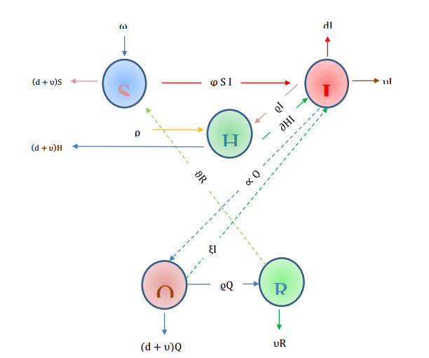
In the present period, a new fast-spreading pandemic disease, officially recognised Coronavirus disease 2019 (COVID-19), has emerged as a serious international threat. We establish a novel mathematical model consists of a system of differential equations representing the population dynamics of susceptible, healthy, infected, quarantined, and recovered individuals. Applying the next generation technique, examine the boundedness, local and global behavior of equilibria, and the threshold quantity. Find the basic reproduction number $R_0$ and discuss the stability analysis of the model. The findings indicate that disease fee equilibria (DFE) are locally asymptotically stable when $R_0 < 1$ and unstable in case $R_0 > 1$. The partial rank correlation coefficient approach (PRCC) is used for sensitivity analysis of the basic reproduction number in order to determine the most important parameter for controlling the threshold values of the model. The linearization and Lyapunov function theories are utilized to identify the conditions for stability analysis. Moreover, solve the model numerically using the well known continuous Galerkin Petrov time discretization scheme. This method is of order 3 in the whole-time interval and shows super convergence of order 4 in the discrete time point. To examine the validity and reliability of the mentioned scheme, solve the model using the classical fourth-order Runge-Kutta technique. The comparison demonstrates the substantial consistency and agreement between the Galerkin-scheme and RK4-scheme outcomes throughout the time interval. Discuss the computational cost of the schemes in terms of time. The investigation emphasizes the precision and potency of the suggested schemes as compared to the other traditional schemes.
Citation: Attaullah, Muhammad Jawad, Sultan Alyobi, Mansour F. Yassen, Wajaree Weera. A higher order Galerkin time discretization scheme for the novel mathematical model of COVID-19[J]. AIMS Mathematics, 2023, 8(2): 3763-3790. doi: 10.3934/math.2023188
In the present period, a new fast-spreading pandemic disease, officially recognised Coronavirus disease 2019 (COVID-19), has emerged as a serious international threat. We establish a novel mathematical model consists of a system of differential equations representing the population dynamics of susceptible, healthy, infected, quarantined, and recovered individuals. Applying the next generation technique, examine the boundedness, local and global behavior of equilibria, and the threshold quantity. Find the basic reproduction number $R_0$ and discuss the stability analysis of the model. The findings indicate that disease fee equilibria (DFE) are locally asymptotically stable when $R_0 < 1$ and unstable in case $R_0 > 1$. The partial rank correlation coefficient approach (PRCC) is used for sensitivity analysis of the basic reproduction number in order to determine the most important parameter for controlling the threshold values of the model. The linearization and Lyapunov function theories are utilized to identify the conditions for stability analysis. Moreover, solve the model numerically using the well known continuous Galerkin Petrov time discretization scheme. This method is of order 3 in the whole-time interval and shows super convergence of order 4 in the discrete time point. To examine the validity and reliability of the mentioned scheme, solve the model using the classical fourth-order Runge-Kutta technique. The comparison demonstrates the substantial consistency and agreement between the Galerkin-scheme and RK4-scheme outcomes throughout the time interval. Discuss the computational cost of the schemes in terms of time. The investigation emphasizes the precision and potency of the suggested schemes as compared to the other traditional schemes.

| [1] |
J. A. Al-Tawfiq, K. Hinedi, J. Ghandour, H. Khairalla, S. Musleh, A. Ujayli, et al., Middle East respiratory syndrome coronavirus: a case-control study of hospitalized patients, Clin. Infect. Dis., 59 (2014), 160–165. https://doi.org/10.1093/cid/ciu226 doi: 10.1093/cid/ciu226

|
| [2] |
E. I. Azhar, S. A. El-Kafrawy, S. A. Farraj, A. M. Hassan, M. S. Al-Saeed, A. M. Hashem, et al., Evidence for camel-to-human transmission of MERS coronavirus, New Engl. J. Med., 370 (2014), 2499–2505. https://doi.org/10.1056/NEJMoa1401505 doi: 10.1056/NEJMoa1401505
|
| [3] |
Y. Kim, S. Lee, C. Chu, S. Choe, S. Hong, Y. Shin, The characteristics of Middle Eastern respiratory syndrome coronavirus transmission dynamics in South Korea, Osong Pub. Health Res. Perspe., 7 (2016), 49–55. https://doi.org/10.1016/j.phrp.2016.01.001 doi: 10.1016/j.phrp.2016.01.001
|
| [4] |
A. H. Abdel-Aty, M. M. Khater, H. Dutta, J. Bouslimi, M. Omri, Computational solutions of the HIV-1 infection of CD4+ T-cells fractional mathematical model that causes acquired immunodeficiency syndrome (AIDS) with the effect of antiviral drug therapy, Chaos Soliton. Fract., 139 (2020), 110092. https://doi.org/10.1016/j.chaos.2020.110092 doi: 10.1016/j.chaos.2020.110092
|
| [5] | W. E. Alnaser, M. Abdel-Aty, O. Al-Ubaydli, Mathematical prospective of coronavirus infections in Bahrain, Saudi Arabia and Egypt, Inf. Sci. Lett., 9 (2020), 1. |
| [6] |
H. A. Rothana, S. N. Byrareddy, The epidemiology and pathogenesis of coronavirus disease (COVID-19) outbreak, J. Autoimmun., 109 (2020), 102433. https://doi.org/10.1016/j.jaut.2020.102433 doi: 10.1016/j.jaut.2020.102433
|
| [7] |
H. Lu, Drug treatment options for the 2019-new coronavirus (2019-nCoV), Biosci. Trend., 14 (2020), 69–71. https://doi.org/10.5582/bst.2020.01020 doi: 10.5582/bst.2020.01020
|
| [8] |
M. Bassetti, A. Vena, D. R. Giacobbe, The novel Chinese coronavirus (2019-nCoV) infections: challenges for fihting the storm, Eur. J. Clin. Invest., 50 (2020), 13209. https://doi.org/10.1111/eci.13209 doi: 10.1111/eci.13209
|
| [9] |
Z. Chen, W. Zhang, Y. Lu, C. Guo, Z. Guo, C. Liao, et al., From SARS-CoV to Wuhan 2019-nCoV outbreak: similarity of early epidemic and prediction of future trends, Cell Host Microbe, 2020. http://dx.doi.org/10.2139/ssrn.3528722 doi: 10.2139/ssrn.3528722
|
| [10] | Worldometer, COVID-19 coronavirus pandemic, 2020. Available from: http://www.worldometers.info/coronavirus/#repro. |
| [11] |
D. Wrapp, N. Wang, K. S. Corbett, J. A. Goldsmith, C. L. Hsieh, O. Abiona, et al., Cryo-EM structure of the 2019-nCoV spike in the prefusion conformation, Science, 367 (2020), 1260–1263. http://dx.doi.org/10.1126/science.abb2507 doi: 10.1126/science.abb2507
|
| [12] |
F. Bozkurt, A. Yousef, D. Baleanu, J. Alzabut, A mathematical model of the evolution and spread of pathogenic coronaviruses from natural host to human host, Chaos Soliton. Fract., 138 (2020), 109931. https://doi.org/10.1016/j.chaos.2020.109931 doi: 10.1016/j.chaos.2020.109931
|
| [13] | World health organization, Coronavirus disease (COVID-2019) situation reports, 2020. Available from: https://www.who.int/emergencies/diseases/novel-coronavirus-2019/situation-reports. |
| [14] |
N. Zhu, D. Zhang, W. Wang, X. Li, B. Yang, J. Song, et al., A novel coronavirus from patients with pneumonia in China, 2019. New England J. Med., 382 (2020), 727–733. https://doi.org/10.1056/NEJMoa2001017 doi: 10.1056/NEJMoa2001017
|
| [15] | NCDC, The Nigeria center for disease control, 2020. Available from: https://covid19.ncdc.gov.ng. |
| [16] |
L. R. Fortuna, M. Tolou-Shams, B. Robles-Ramamurthy, M. V. Porche, Inequity and the disproportionate impact of COVID-19 on communities of color in the United States: the need for a trauma-informed social justice response, Psychol. Trauma Theory Res. Pract. Policy, 12 (2020), 443–445. https://doi.org/10.1037/tra0000889 doi: 10.1037/tra0000889
|
| [17] |
P. Sunthrayuth, M. A. Khan, F. S. Alshammari, Mathematical Modeling to determine the fifth wave of COVID-19 in South Africa, BioMed Res. Int., 2022 (2022), 9932483. https://doi.org/10.1155/2022/9932483 doi: 10.1155/2022/9932483
|
| [18] |
G. M. Vijayalakshmi, B. P. Roselyn, A fractal fractional order vaccination model of COVID-19 pandemic using Adam's moulton analysis, Results Control Optim., 8 (2022), 100144. https://doi.org/10.1016/j.rico.2022.100144 doi: 10.1016/j.rico.2022.100144
|
| [19] |
R. Cerqueti, V. Ficcadenti, Combining rank-size and k-means for clustering countries over the COVID-19 new deaths per million, Chaos Soliton. Fract., 158 (2022), 111975. https://doi.org/10.1016/j.chaos.2022.111975 doi: 10.1016/j.chaos.2022.111975
|
| [20] | ECDC, Data on the daily number of new reported COVID-19 cases and deaths by EU/EEA country, 2020. Available from: https://www.ecdc.europa.eu/en/publications-data/data-daily-new-cases-covid-19-eueea-country. |
| [21] | R. Ranjan, H. S. Prasad, A fitted finite difference scheme for solving singularly perturbed two point boundary value problems, Inf. Sci. Lett., 9 (2020), 65–73. |
| [22] |
F. Brauer, Mathematical epidemiology: past, present, and future, Infect. Dis. Model., 2 (2017), 113–127. https://doi.org/10.1016/j.idm.2017.02.001 doi: 10.1016/j.idm.2017.02.001
|
| [23] |
P. D. En'Ko, On the course of epidemics of some infectious diseases, Int. J. Epidemiol., 18 (1989), 749–755. https://doi.org/10.1093/ije/18.4.749 doi: 10.1093/ije/18.4.749
|
| [24] |
A. R. Hadhoud, Quintic non-polynomial spline method for solving the time fractional biharmonic equation, Appl. Math. Inf. Sci., 13 (2019), 507–513. http://dx.doi.org/10.18576/amis/130323 doi: 10.18576/amis/130323
|
| [25] |
J. Ereu, J. Gimenez, L. Perez, On solutions of nonlinear integral equations in the space of functions of Shiba-bounded variation, Appl. Math. Inf. Sci., 14 (2020), 393–404. http://dx.doi.org/10.18576/amis/140305 doi: 10.18576/amis/140305
|
| [26] | C. Castillo-Chavez, S. Blower, P. van den Driessche, D. Kirschner, A. Yakubu, Mathematical approaches for emerging and reemerging infectious diseases: an introduction, Berlin: Springer 2002. |
| [27] |
D. Kumar D, J. Singh, M. A. Qurashi, D. Baleanu, A new fractional SIRS-SI malaria disease model with application of vaccines, antimalarial drugs, and spraying, Adv. Differ. Equ., 278 (2019). https://doi.org/10.1186/s13662-019-2199-9 doi: 10.1186/s13662-019-2199-9
|
| [28] |
A. S. Shaikh, I. N. Shaikh, K. S. Nisar, A mathematical model of COVID-19 using fractional derivative: Outbreak in India with dynamics of transmission and control, Adv. Differ. Equ., 373 (2020). https://doi.org/10.1186/s13662-020-02834-3 doi: 10.1186/s13662-020-02834-3
|
| [29] |
M. A. Khan, A. Atangana, Modeling the dynamics of novel coronavirus (2019-nCov) with fractional derivative, Alex. Eng. J., 59 (2020), 2379–2389. https://doi.org/10.1016/j.aej.2020.02.033 doi: 10.1016/j.aej.2020.02.033
|
| [30] |
F. Ndairou, I. Area, J. J. Nieto, D. F. Torres. Mathematical modeling of COVID-19 transmission dynamics with a case study of Wuhan, Chaos Soliton. Fract., 135 (2020), 109846. https://doi.org/10.1016/j.chaos.2020.109846 doi: 10.1016/j.chaos.2020.109846
|
| [31] |
A. Pan, L. Liu, C. Wang, H. Guo, X. Hao, Q. Wang, et al., A conceptual model for the coronavirus disease 2019 (COVID-19) outbreak in Wuhan, China with individual reaction and governmental action, Int. J. Infect. Dis., 93 (2020), 211–216. https://doi.org/10.1016/j.ijid.2020.02.058 doi: 10.1016/j.ijid.2020.02.058
|
| [32] |
M. S. Abdo, K. Shah, H. A. Wahash, S. K. Panchal, On a comprehensive model of the novel coronavirus (COVID-19) under Mittag-Leffler derivative, Chaos Soliton. Fract., 135 (2020), 109867. https://doi.org/10.1016/j.chaos.2020.109867 doi: 10.1016/j.chaos.2020.109867
|
| [33] |
M. Yousaf, S. Zahir, M. Riaz, S. M. Hussain, K. Shah, Statistical analysis of forecasting COVID-19 for upcoming month in Pakistan, Chaos Soliton. Fract., 138 (2020), 109926. https://doi.org/10.1016/j.chaos.2020.109926 doi: 10.1016/j.chaos.2020.109926
|
| [34] |
A. Atangana, Modelling the spread of COVID-19 with new fractal-fractional operators: Can the lockdown save mankind before vaccination, Chaos Soliton. Fract., 136 (2020), 109860. https://doi.org/10.1016/j.chaos.2020.109860 doi: 10.1016/j.chaos.2020.109860
|
| [35] |
D. Okuonghae, A. Omame, Analysis of a mathematical model for COVID-19 population dynamics in Lagos, Nigeria, Chaos Soliton. Fract., 139 (2020), 110032. https://doi.org/10.1016/j.chaos.2020.110032 doi: 10.1016/j.chaos.2020.110032
|
| [36] |
R. O. Ogundokun, A. F. Lukman, G. B. Kibria, J. B. Awotunde, B. B. Aladeitan, Predictive modelling of COVID-19 confirmed cases in Nigeria, Infec. Dis. Model., 5 (2020), 543–548. https://doi.org/10.1016/j.idm.2020.08.003 doi: 10.1016/j.idm.2020.08.003
|
| [37] |
M. S. Abdo MS, K. Shah, H. A. Wahash, S. K. Panchal, On a comprehensive model of the novel coronavirus (COVID-19) under Mittag-Leffler derivative, Chaos Soliton. Fract., 135 (2020), 109867. https://doi.org/10.1016/j.chaos.2020.109867 doi: 10.1016/j.chaos.2020.109867
|
| [38] |
O. A. Adegboye, A. I. Adekunle, E. Gayawan, Early transmission dynamics of novel coronavirus (COVID-19) in Nigeria, Int. J. Env. Res. Pub. He., 17 (2020), 3054. https://doi.org/10.3390/ijerph17093054 doi: 10.3390/ijerph17093054
|
| [39] | W. Ajisegiri, O. Odusanya, R. Joshi, COVID-19 outbreak situation in Nigeria and the need for effective engagement of community health workers for epidemic response, Glob. Biosecur., 2 (2020). |
| [40] |
C. Anastassopoulou, L. Russo, A. Tsakris, C. Siettos, Data-based analysis, modelling and forecasting of the COVID-19 outbreak, PLoS One, 15 (2020). https://doi.org/10.1371/journal.pone.0230405 doi: 10.1371/journal.pone.0230405
|
| [41] |
D. Fanelli, F. Piazza, Analysis and forecast of COVID-19 spreading in China, Italy and France, Chaos Soliton. Fract., 134 (2020), 109761. https://doi.org/10.1016/j.chaos.2020.109761 doi: 10.1016/j.chaos.2020.109761
|
| [42] |
W. C. Roda, M. B. Varughese, D. Han, M. Y. Li, Why is it difficult to accurately predict the COVID-19 epidemic, Infect. Dis. Model., 5 (2020), 271–281. https://doi.org/10.1016/j.idm.2020.03.001 doi: 10.1016/j.idm.2020.03.001
|
| [43] |
M. A. Al-Qaness, A. A. Ewees, H. Fan, M. Abd El Aziz, Optimization method for forecasting confirmed cases of COVID-19 in China, J. Clin. Med., 9 (2020), 674. https://doi.org/10.3390/jcm9030674 doi: 10.3390/jcm9030674
|
| [44] |
W. Wei, J. Jiang, H. Liang, L. Gao, B. Liang, J. Huang, et al., Application of a combined model with autoregressive integrated moving average (ARIMA) and generalized regression neural network (GRNN) in forecasting hepatitis incidence in Heng County, China, PLoS One, 11 (2016). https://doi.org/10.1371/journal.pone.0156768 doi: 10.1371/journal.pone.0156768
|
| [45] |
O. Nave, U. Shemesh, I. HarTuv, Applying Laplace Adomian decomposition method (LADM) for solving a model of COVID-19, Comput. Method. Biomec., 24 (2021), 1618–1628. https://doi.org/10.1080/10255842.2021.1904399 doi: 10.1080/10255842.2021.1904399
|
| [46] |
H. Schiøler, T. Knudsen, R. F. Brøndum, J. Stoustrup, M. Bøgsted, Mathematical modelling of SARS-CoV-2 variant outbreaks reveals their probability of extinction, Sci. Rep., 11 (2021), 24498. https://doi.org/10.1038/s41598-021-04108-8 doi: 10.1038/s41598-021-04108-8
|
| [47] |
S. Ahmad, S. Owyed, A. H. Abdel-Aty, E. E. Mahmoud, K. Shah, H. Alrabaiah, Mathematical analysis of COVID-19 via new mathematical model, Chaos Soliton. Fract., 143 (2021), 110585. https://doi.org/10.1016/j.chaos.2020.110585 doi: 10.1016/j.chaos.2020.110585
|
| [48] | O. J. Peter, S. Qureshi, A. Yusuf, M. Al-Shomrani, A. A. Idowu, A new mathematical model of COVID-19 using real data from Pakistan, Results Phys., 24 (2021), 104098. |
| [49] |
P. van den Driessche, J. Watmough, Reproduction numbers and sub-threshold endemic equilibria for compartmental models of disease transmission, Math. Biosci., 180 (2022), 29–48. https://doi.org/10.1016/S0025-5564(02)00108-6 doi: 10.1016/S0025-5564(02)00108-6
|
| [50] |
C. Castillo-Chavez, B. Song, Dynamical models of tuberculosis and their applications, Math. Biosci, Eng., 1 (2004), 361. https://doi.org/10.3934/mbe.2004.1.361 doi: 10.3934/mbe.2004.1.361
|
| [51] |
O. Sharomi, C. N. Podder, A. B. Gumel, E. H. Elbasha, J. Watmough, Role of incidence function in vaccine-induced backward bifurcation in some HIV models, Math. Biosci., 210 (2007), 436–463. https://doi.org/10.1016/j.mbs.2007.05.012 doi: 10.1016/j.mbs.2007.05.012
|
| [52] |
F. Schieweck, A-stable discontinuous Galerkin-Petrov time discretization of higher order, J. Numer. Math., 18 (2010), 25–57. https://doi.org/10.1515/jnum.2010.002 doi: 10.1515/jnum.2010.002
|
| [53] |
S. Hussain, F. Schieweck, S. Turek, Higher order Galerkin time discretizations and fast multigrid solvers for the heat equation, J. Numer. Math., 19 (2011), 41–61. https://doi.org/10.1515/jnum.2011.003 doi: 10.1515/jnum.2011.003
|
| [54] |
S. Hussain, F. Schieweck, S. Turek, A note on accurate and efficient higher order Galerkin time stepping schemes for the nonstationary Stokes equations, Open Numer. Method. J., 4 (2012), 35–45. https://doi.org/10.2174/1876389801204010035 doi: 10.2174/1876389801204010035
|
| [55] |
S. Hussain, F. Schieweck, S. Turek, An efficient and stable finite element solver of higher order in space and time for nonstationary incompressible flow, Int. J. Numer. Meth. Fl., 73 (2013), 927–952. https://doi.org/10.1002/fld.3831 doi: 10.1002/fld.3831
|
| [56] | G. Matthies, F. Schieweck, Higher order variational time discretizations for nonlinear systems of ordinary differential equations, Otto Von Guericke Universität Magdeburg, 2011, 1–30. |
| [57] |
Attaullah, M. Sohaib, Mathematical modeling and numerical simulation of HIV infection model, Results Appl. Math., 7 (2020), 100118. https://doi.org/10.1016/j.rinam.2020.100118 doi: 10.1016/j.rinam.2020.100118
|
| [58] | H. Leal, L. Hernandez-Martinez, Y. Khan, V. Jimenez-Fernandez, U. Filobello-Nino, A. Diaz-Sanchez, et al., Mul-tistage HPM applied to path tracking damped oscillations of a model for HIV infection of CD4+ T-cells, British J. Math. Comput. Sci., 8 (2014), 1035–1047. |
| [59] |
Attaullah, R. Jan, S. Yüzbaşı, Dynamical behaviour of HIV infection with the influence of variable source term through Galerkin method, Chaos Soliton. Fract., 152 (2021), 111429. https://doi.org/10.1016/j.chaos.2021.111429 doi: 10.1016/j.chaos.2021.111429
|
| [60] | A. Aziz, P. Monk, Continuous finite elements in space and time for the heat equation, Math. Comput., 52 (1989), 255–274. |


Figures(10) / Tables(3)

Attaullah, Muhammad Jawad, Sultan Alyobi, Mansour F. Yassen, Wajaree Weera. A higher order Galerkin time discretization scheme for the novel mathematical model of COVID-19[J]. AIMS Mathematics, 2023, 8(2): 3763-3790. doi: 10.3934/math.2023188


 DownLoad: