Solving the time-fractional inverse Burger equation involving fractional Heydari-Hosseininia derivative

Mohammad Partohaghighi; Ali Akgül; Jihad Asad; Rania Wannan; Mohammad Partohaghighi; Ali Akgül; Jihad Asad; Rania Wannan

doi:10.3934/math.2022959

AIMS Mathematics

2022, Volume 7, Issue 9: 17403-17417. doi: 10.3934/math.2022959

Previous Article Next Article

Research article Special Issues

Solving the time-fractional inverse Burger equation involving fractional Heydari-Hosseininia derivative

1.
Department of Mathematics, University of Clarkson, New York, USA
2.
Department of Mathematics, Art and Science Faculty, 56100 Siirt, Siirt university, Turkey
3.
Department Of Physics, Faculty of Applied Sciences, Palestine Technical University- Kadoorie, Tulkarm, Palestine
4.
Department of Applied Mathematics, Faculty of Applied Sciences, Palestine Technical University- Kadoorie, Tulkarm, Palestine

Received: 27 March 2022 Revised: 26 May 2022 Accepted: 09 June 2022 Published: 28 July 2022
MSC : 34K37, 35R11, 90C32

In this paper, we present a powerful numerical scheme based on energy boundary functions to get the approximate solutions of the time-fractional inverse Burger equation containing HH-derivative.This problem has never been investigated earlier so, this is our motivation to work on this important problem. Some numerical examples are presented to verify the efficiency of the presented technique. Graphs of the exact and numerical solutions along with the plot of absolute error are provided for each example. Tables are given to see and compare the results point by point for each example.
- Optimization,
- fractional inverse Burger equation,
- Heydari-Hosseininia derivative
Citation: Mohammad Partohaghighi, Ali Akgül, Jihad Asad, Rania Wannan. Solving the time-fractional inverse Burger equation involving fractional Heydari-Hosseininia derivative[J]. AIMS Mathematics, 2022, 7(9): 17403-17417. doi: 10.3934/math.2022959

Related Papers:

Abstract

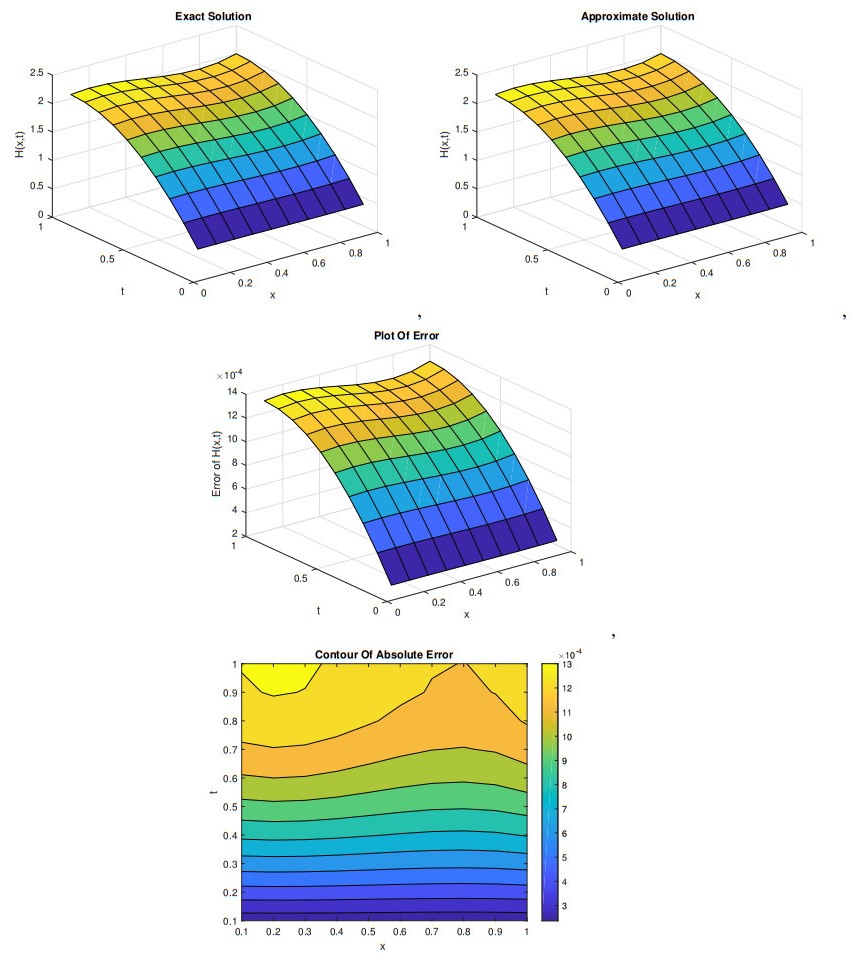
In this paper, we present a powerful numerical scheme based on energy boundary functions to get the approximate solutions of the time-fractional inverse Burger equation containing HH-derivative.This problem has never been investigated earlier so, this is our motivation to work on this important problem. Some numerical examples are presented to verify the efficiency of the presented technique. Graphs of the exact and numerical solutions along with the plot of absolute error are provided for each example. Tables are given to see and compare the results point by point for each example.

References

[1]	Y. T. Gu, P. Zhuang, F. Liu, An advanced implicit meshless approach for the non-linear anomalous subdiffsion equation, Comput. Model. Eng. Sci., 56 (2010), 303–333. http://dx.doi.org/10.3970/cmes.2010.056.303 doi: 10.3970/cmes.2010.056.303
[2]	C. S. Liu, The fictitious time integration method to solve the space- and time-fractional Burgers equations, Comput. Mater. Contin., 15 (2011), 221–240. http://dx.doi.org/10.2298/TSCI190421365P doi: 10.2298/TSCI190421365P
[3]	D. Li, C. Zhang, M. Ran, A linear finite difference scheme for generalized time fractional Burgers equation, Appl. Math. Model., 40 (2016), 6069–6081. https://doi.org/10.1016/j.apm.2016.01.043 doi: 10.1016/j.apm.2016.01.043
[4]	M. Shakeel, Q. M. Ul-Hassan, J. Ahmad, T. Naqvi, Exact solutions of the time fractional BBM-Burger equation by novel (G$\prime$/G)-expansion method, Adv. Math. Phys., 2 (2014), 15pages. http://dx.doi.org/10.1155/2014/181594 doi: 10.1155/2014/181594
[5]	A. El-Ajou, O. A. Arqub, S. Momani, Approximate analytical solution of the nonlinear fractional KdV–Burgers equation: A new iterative algorithm, J. Comput. Phys., 293 (2014), 81–95. http://dx.doi.org/10.1016/j.jcp.2014.08.004 doi: 10.1016/j.jcp.2014.08.004
[6]	M. Rawashdeh, An efficient approach for time-fractional damped Burger and time-sharma-tasso-Olver equations using the FRDTM, Appl. Math. Inf. Sci., 9 (2015), 1239–1246. http://dx.doi.org/10.12785/amis/090317 doi: 10.12785/amis/090317
[7]	M. Rawashdeh, A reliable method for the space–time fractional Burgers and time-fractional Cahn-Allen equations via the FRDTM, Adv. Differ. Equ., 2017 (2017), 99. https://advancesindifferenceequations.springeropen.com/articles/10.1186/s13662-017-1148-8
[8]	A. Esen, O. Tasbozan, Numerical solution of time fractional Burgers equation by cubic B-spline finite elements Method, Mediterr. J. Math., 13 (2016), 1325–1337. http://dx.doi.org/10.1007/s00009-015-0555-x doi: 10.1007/s00009-015-0555-x
[9]	K. Saad, E. H. Al-Sharif, Analytical study for time and time-space fractional Burgers' equation, Adv. Differ. Equ., 2017 (2017). http://dx.doi.org/10.1186/s13662-017-1358-0
[10]	S. S. Ray, A new coupled fractional reduced differential transform method for the numerical solutions of (2+1)–Dimensional time fractional coupled Burger equations, Model. Simul. Eng., 2014 (2014), 12 pages. https://doi.org/10.1155/2014/960241 doi: 10.1155/2014/960241
[11]	K. Saad, A. Atangana, D. Baleanu, New fractional derivatives with non-singular kernel applied to the burgers equation, Chaos, 28 (2018). http://dx.doi.org/10.1063/1.5026284
[12]	Y. Xu, O. Agrawal, Numerical solutions and analysis of diffusion for new generalized fractional burgers equation, Fract. Calc. Appl. Anal., 16 (2013), 709–736. http://dx.doi.org/10.2478/s13540-013-0045-4 doi: 10.2478/s13540-013-0045-4
[13]	N. Bildik, S. Deniz, Solving the Burgers' and regularized long wave equations using the new perturbation iteration technique, Numer. Meth. Part. D. E., 34 (2018), 1489–1501. https://doi.org/10.1002/num.22214 doi: 10.1002/num.22214
[14]	S. Deniz, A. Konuralp, M. De la Sen, Optimal perturbation iteration method for solving fractional model of damped Burgers' equation, Symmetry, 12 (2020), 958. https://doi.org/10.3390/sym12060958 doi: 10.3390/sym12060958
[15]	H. Li, Y. Wu, Artificial boundary conditions for nonlinear time fractional Burgers' equation on unbounded domains, Appl. Math. Lett., 120 (2021). https://doi.org/10.1016/j.aml.2021.107277
[16]	L. Li, D. Li, Exact solutions and numerical study of time fractional Burgers' equations, Appl. Math. Lett., 100 (2020). https://doi.org/10.1016/j.aml.2019.106011
[17]	M. H. Heydari, M. Hosseininia, A new variable‑order fractional derivative with non‑singular Mittag-Leffler kernel: Application to variable‑order fractional version of the 2D Richard equation, Eng. Comput-Germany, 8 (2022), 1–12. https://link.springer.com/article/10.1007/s00366-020-01121-9
[18]	C. Liu, B. Li, Forced and free vibrations of composite beams solved by an energetic boundary functions collocation method, Math. Comput. Simul., 177 (2020), 152–168. https://doi.org/10.1016/j.matcom.2020.04.020 doi: 10.1016/j.matcom.2020.04.020
[19]	C. Liu, H. Chen, J. Chang, Identifying heat conductivity and source functions for a nonlinear convective-diffusive equation by energetic boundary functional methods, Numer. Heat Tr., B-Fund., 78 (2020), 248–264. https://doi.org/10.1080/10407790.2020.1777790 doi: 10.1080/10407790.2020.1777790
[20]	C. Liu, An energetic boundary functional method for solving the inverse source problems of 2D nonlinear elliptic equations, Eng. Anal. Bound. Elem., 118 (2020), 204–215. https://doi.org/10.1016/j.enganabound.2020.06.009 doi: 10.1016/j.enganabound.2020.06.009
[21]	C. Liu, An energetic boundary functional method for solving the inverse heat conductivity problems in arbitrary plane domains, Int. J. Heat Mass Tran., 151 (2020). https://doi.org/10.1016/j.ijheatmasstransfer.2020.119418
[22]	C. Liu, B. Li, S. Liu, Solving a nonlinear inverse Sturm–Liouville problem with nonlinear convective term using a boundary functional method, Inverse Probl. Sci. En., 28 (2019), 1135–1153. https://doi.org/10.1080/17415977.2019.1705804 doi: 10.1080/17415977.2019.1705804
[23]	L. Qiu, W. Chen, F. Wang, C. Liu, Q. Hua, Boundary function method for boundary identification in two-dimensional steady-state nonlinear heat conduction problems, Eng. Anal. Bound. Elem., 103 (2019), 101–108. https://doi.org/10.1016/j.enganabound.2019.03.004 doi: 10.1016/j.enganabound.2019.03.004
[24]	C. Liu, J. Chang, Recovering a source term in the time-fractional Burgers equation by an energy boundary functional equation, Appl. Math. Lett., 79 (2018), 138–145. https://doi.org/10.1016/j.aml.2017.12.010 doi: 10.1016/j.aml.2017.12.010
[25]	C. Liu, Solving inverse coefficient problems of non-uniform fractionally diffusive reactive material by a boundary functional method, Int. J. Heat Mass Tran., 116 (2018), 587–598. https://doi.org/10.1016/j.ijheatmasstransfer.2017.08.124 doi: 10.1016/j.ijheatmasstransfer.2017.08.124
[26]	C. Liu, B. Li, Reconstructing a second-order Sturm–Liouville operator by an energetic boundary function iterative method, Appl. Math. Lett., 73 (2017), 49–55. https://doi.org/10.1016/j.aml.2017.04.023 doi: 10.1016/j.aml.2017.04.023

Reader Comments

Your name:*

Email:*
© 2022 the Author(s), licensee AIMS Press. This is an open access article distributed under the terms of the Creative Commons Attribution License (http://creativecommons.org/licenses/by/4.0)