Soliton solutions of conformable time-fractional perturbed Radhakrishnan-Kundu-Lakshmanan equation

Chun Huang; Zhao Li; Chun Huang; Zhao Li

doi:10.3934/math.2022797

AIMS Mathematics

2022, Volume 7, Issue 8: 14460-14473. doi: 10.3934/math.2022797

Previous Article Next Article

Research article Special Issues

Soliton solutions of conformable time-fractional perturbed Radhakrishnan-Kundu-Lakshmanan equation

Chun Huang ¹,
Zhao Li ^{2
,
,}

1.
Faculty of Education, Sichuan Vocational and Technical College, Suining 629000, China
2.
College of Computer Science, Chengdu University, Chengdu 610106, China

Received: 08 April 2022 Revised: 24 May 2022 Accepted: 30 May 2022 Published: 06 June 2022
MSC : 35C05, 35C07, 35R11

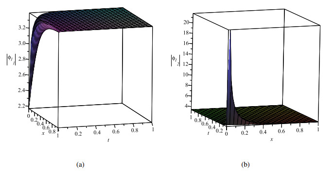
In this paper, our main purpose is to study the soliton solutions of conformable time-fractional perturbed Radhakrishnan-Kundu-Lakshmanan equation. New soliton solutions have been obtained by the extended $ (G'/G) $-expansion method, first integral method and complete discrimination system for the polynomial method, respectively. The solutions we obtained mainly include hyperbolic function solutions, solitary wave solutions, Jacobi elliptic function solutions, trigonometric function solutions and rational function solutions. Moreover, we draw its three-dimensional graph.
Citation: Chun Huang, Zhao Li. Soliton solutions of conformable time-fractional perturbed Radhakrishnan-Kundu-Lakshmanan equation[J]. AIMS Mathematics, 2022, 7(8): 14460-14473. doi: 10.3934/math.2022797

Related Papers:

Abstract

In this paper, our main purpose is to study the soliton solutions of conformable time-fractional perturbed Radhakrishnan-Kundu-Lakshmanan equation. New soliton solutions have been obtained by the extended $ (G'/G) $-expansion method, first integral method and complete discrimination system for the polynomial method, respectively. The solutions we obtained mainly include hyperbolic function solutions, solitary wave solutions, Jacobi elliptic function solutions, trigonometric function solutions and rational function solutions. Moreover, we draw its three-dimensional graph.

References

[1]	T. Han, Z. Li, X. Zhang, Bifurcation and new exact traveling wave solutions to time-space coupled fractional nonlinear Schrödinger equation, Phys. Lett. A, 395 (2021), 127217. http://dx.doi.org/10.1016/j.physleta.2021.127217 doi: 10.1016/j.physleta.2021.127217
[2]	M. Ekicia, M. Mirzazadehb, A. Sonmezoglua, M. Ullah, M. Asma, Q. Zhou, et al., Dispersive optical solitons with Schrödinger-Hirota equation by extended trial equation method, Optik, 136 (2017), 451–461. http://dx.doi.org/10.1016/j.ijleo.2017.02.042 doi: 10.1016/j.ijleo.2017.02.042
[3]	S. Ray, Dispersive optical solitons of time-fractional Schrödinger-Hirota equation in nonlinear optical fibers, Physica A, 537 (2020), 122619. http://dx.doi.org/10.1016/j.physa.2019.122619 doi: 10.1016/j.physa.2019.122619
[4]	B. Kilic, M. Inc, Optical solitons for the Schrödinger-Hirota equation with power law nonlinearity by the Bäcklund transformation, Optik, 138 (2017), 64–67. http://dx.doi.org/10.1016/j.ijleo.2017.03.017 doi: 10.1016/j.ijleo.2017.03.017
[5]	H. Zhang, R. Hu, M. Zhang, Darboux transformation and dark soliton solution for the defocusing Sasa-Satsuma equation, Appl. Math. Lett., 69 (2017), 101–105. http://dx.doi.org/10.1016/j.aml.2017.02.012 doi: 10.1016/j.aml.2017.02.012
[6]	M. Shehata, H. Rezazadeh, E. Zahran, E. Tala-Tebue, A. Bekir, New optical soliton solutions of the perturbed Fokas-Lenells equation, Commun. Theor. Phys., 71 (2019), 1275–1280. http://dx.doi.org/10.1088/0253-6102/71/11/1275 doi: 10.1088/0253-6102/71/11/1275
[7]	M. Eslami, M. Mirzazadeh, B. Fathi Vajargah, A. Biswas, Optical solitons for the resonant nonlinear Schrödinger's equation with time-dependent coefficients by the first integral method, Optik, 125 (2014), 3107–3116. http://dx.doi.org/10.1016/j.ijleo.2014.01.013 doi: 10.1016/j.ijleo.2014.01.013
[8]	S. Rizvi, A. Seadawy, U. Akram, M. Youni, A. Althobaiti, Solitary wave solutions along with Painleve analysis for the Ablowitz-Kaup-Newell-Segur water waves equation, Mod. Phys. Lett. B, 36 (2022), 2150548. http://dx.doi.org/10.1142/S0217984921505485 doi: 10.1142/S0217984921505485
[9]	S. Rizvi, A. Seadawy, K. Ali, M. Ashraf, S. Althubiti, Multiple lump and interaction solutions for fifth-order variable coefficient nonlinear-Schrödinger dynamical equation, Opt. Quant. Electron., 54 (2022), 154. http://dx.doi.org/10.1007/s11082-022-03532-y doi: 10.1007/s11082-022-03532-y
[10]	S. Rizvi, A. Seadawy, K. Ali, M. Younis, M. Ashraf, Multiple lump and rogue wave for time fractional resonant nonlinear Schrödinger equation under parabolic law with weak nonlocal nonlinearity, Opt. Quant. Electron., 54 (2022), 212. http://dx.doi.org/10.1007/s11082-022-03606-x doi: 10.1007/s11082-022-03606-x
[11]	U. Akram, A. Seadawy, S. Rizvi, B. Mustafa, Applications of the resonanat nonlinear Schrödinger equation with self steeping phenomena for chirped periodic waves, Opt. Quant. Electron., 54 (2022), 256. http://dx.doi.org/10.1007/s11082-022-03525-x doi: 10.1007/s11082-022-03525-x
[12]	A. Bashira, A. Seadawyb, S. Rizvia, I. Alia, S. Althubitic, Dispersive dromions, conserved densities and fluxes with integrability via P-test for couple of nonlinear dynamical system, Results Phys., 33 (2022), 105151. http://dx.doi.org/10.1016/j.rinp.2021.105151 doi: 10.1016/j.rinp.2021.105151
[13]	A. Seadawya, M. Younisb, M. Baberc, M. Iqbald, S. Rizvie, Nonlinear acoustic wave structures to the Zabolotskaya-Khokholov dynamical model, J. Geom. Phys., 175 (2022), 104474. http://dx.doi.org/10.1016/j.geomphys.2022.104474 doi: 10.1016/j.geomphys.2022.104474
[14]	A. Seadawya, S. Ahmedb, S. Rizvib, K. Ali, Various forms of lumps and interaction solutions to generalized Vakhnenko Parkes equation arising from high-frequency wave propagation in electromagnetic physics, J. Geom. Phys., 176 (2022), 104507. http://dx.doi.org/10.1016/j.geomphys.2022.104507 doi: 10.1016/j.geomphys.2022.104507
[15]	A. Seadawya, U. Akramb, S. Rizvib, Dispersive optical solitons along with integrability test and one soliton transformation for saturable cubic-quintic nonlinear media with nonlinear dispersion, J. Geom. Phys., 177 (2022), 104521. http://dx.doi.org/10.1016/j.geomphys.2022.104521 doi: 10.1016/j.geomphys.2022.104521
[16]	S. Rizvi, A. Seadawy, U. Akram, New dispersive optical soliton for an nonlinear Schrödinger equation with Kudryashov law of refractive index along with P-test, Opt. Quant. Electron., 54 (2022), 310. http://dx.doi.org/10.1007/s11082-022-03711-x doi: 10.1007/s11082-022-03711-x
[17]	A. Seadawya, A. Alib, W. Albarakati, Analytical wave solutions of the (2+1)-dimensional first integro-differential Kadomtsev-Petviashivili hierarchy equation by using modified mathematical methods, Results Phys., 15 (2019), 102775. http://dx.doi.org/10.1016/j.rinp.2019.102775 doi: 10.1016/j.rinp.2019.102775
[18]	A. Seadawy, D. Kumar, A. Chakrabarty, Dispersive optical soliton solutions for the hyperbolic and cubic-quintic nonlinear Schrödinger equations via the extended sinh-Gordon equation expansion method, Eur. Phys. J. Plus, 133 (2018), 182. http://dx.doi.org/10.1140/epjp/i2018-12027-9 doi: 10.1140/epjp/i2018-12027-9
[19]	N. Çelik, A. Seadawy, Y. Sağlam Özkan, E. Yaşar, A model of solitary waves in a nonlinear elastic circular rod: abundant different type exact solutions and conservation laws, Chaos Soliton. Fract., 143 (2021), 110486. http://dx.doi.org/10.1016/j.chaos.2020.110486 doi: 10.1016/j.chaos.2020.110486
[20]	H. Rehman, N. Ullah, M. Imran, Optical solitons of Biswas-Arshed equation in birefringent fibers using extended direct algebraic method, Optik, 226 (2021), 165378. http://dx.doi.org/10.1016/j.ijleo.2020.165378 doi: 10.1016/j.ijleo.2020.165378
[21]	H. Rehman, N. Ullah, M. Imran, Highly dispersive optical solitons using Kudryashov's method, Optik, 199 (2029), 163349. http://dx.doi.org/10.1016/j.ijleo.2019.163349 doi: 10.1016/j.ijleo.2019.163349
[22]	S. Singh, Solutions of Kudryashov-Sinelshchikov equation and generalized Radhakrishnan-Kundu-Lakshmanan equation by the first integral method, Int. J. Phys. Res., 4 (2016), 37–42. http://dx.doi.org/10.14419/IJPR.V4I2.6202 doi: 10.14419/IJPR.V4I2.6202
[23]	B. Ghanbari, M. Inc, A. Yusuf, M. Bayram, Exact optical solitons of Radhakrishnan-Kundu-Lakshmanan equation with Kerr law nonlinearity, Mod. Phys. Lett. B, 33 (2019), 1950061. http://dx.doi.org/10.1142/S0217984919500611 doi: 10.1142/S0217984919500611
[24]	O. Gonz$\acute{a}$lez-Gaxiola, A. Biswas, Optical solitons with Radhakrishnan-Kundu-Lakshmanan equation by Laplace-Adomian decomposition method, Optik, 179 (2019), 434–442. http://dx.doi.org/10.1016/j.ijleo.2018.10.173 doi: 10.1016/j.ijleo.2018.10.173
[25]	J. Zhang, S. Li, H. Geng, Bifurcations of exact travelling wave solutions foe the generalized R-K-L equation, J. Appl. Anal. Comput., 6 (2016), 1205–1210. http://dx.doi.org/ 10.11948/2016080 doi: 10.11948/2016080
[26]	N. Kudryashov, D. Safonova, A. Biswas, Painlevé analysis and a solution to the traveling wave reduction of the Radhakrishnan-Kundu-Lakshmanan equation, Regul. Chaot. Dyn., 24 (2019), 607–614. http://dx.doi.org/10.1134/S1560354719060029 doi: 10.1134/S1560354719060029
[27]	D. Lu, A. Seadawy, M. Khater, Dispersive optical soliton solutions of the generalized Radhakrishnan-Kundu-Lakshmanan dynamical equation with power law nonlinearity and its applications, Optik, 164 (2018), 54–64. http://dx.doi.org/10.1016/j.ijleo.2018.02.082 doi: 10.1016/j.ijleo.2018.02.082
[28]	N. Raza, A. Javid, Dynamics of optical solitons with Radhakrishnan-Kundu-Lakshmanan model via two reliable integration schemes, Optik, 178 (2019), 557–566. http://dx.doi.org/10.1016/j.ijleo.2018.09.133 doi: 10.1016/j.ijleo.2018.09.133
[29]	A. Biswas, Y. Yildirim, E. Yasar, M. Mahmood, A. Alshomrani, Q. Zhou, et al., Optical soliton perturbation for Radhakrishnan-Kundu-Lakshmanan equation with a couple of integration schemes, Optik, 163 (2018), 126–136. http://dx.doi.org/10.1016/j.ijleo.2018.02.109 doi: 10.1016/j.ijleo.2018.02.109
[30]	T. Sulaiman, H. Bulut, G. Yel, S. Atas, Optical solitons to the fractional perturbed Radhakrishnan-Kundu-Lakshmanan model, Opt. Quant. Electron., 50 (2018), 372. http://dx.doi.org/10.1007/s11082-018-1641-7 doi: 10.1007/s11082-018-1641-7
[31]	T. Sulaiman, H. Bulut, The solitary wave solutions to the fractional Radhakrishnan-Kundu-Lakshmanan model, Int. J. Mod. Phys. B, 33 (2019), 1950370. http://dx.doi.org/10.1142/S0217979219503703 doi: 10.1142/S0217979219503703
[32]	B. Ghanbari, J. Gómez-Aguilar, The generalized exponential rational function method for Radhakrishnan-Kundu-Lakshmanan equation with $\beta$-conformable time derivative, Rev. Mex. Fis., 65 (2019), 503–518. http://dx.doi.org/10.31349/revmexfis.65.503 doi: 10.31349/revmexfis.65.503

Reader Comments

Your name:*

Email:*
© 2022 the Author(s), licensee AIMS Press. This is an open access article distributed under the terms of the Creative Commons Attribution License (http://creativecommons.org/licenses/by/4.0)