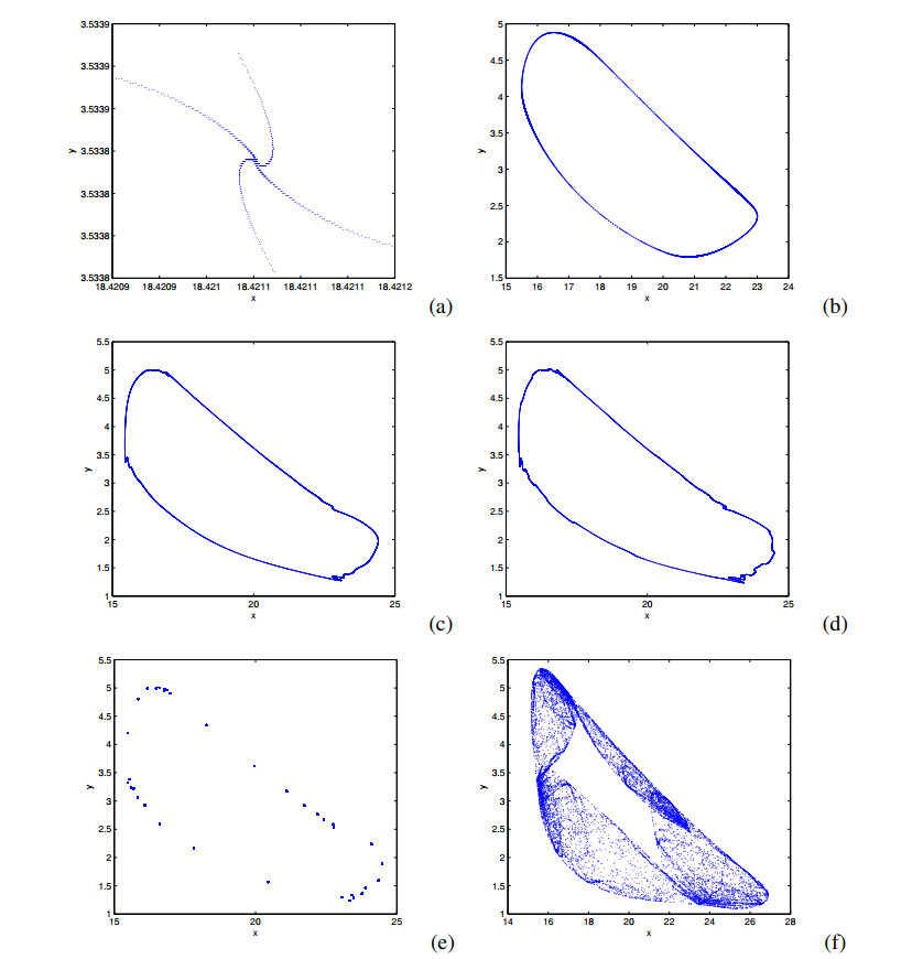
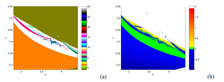
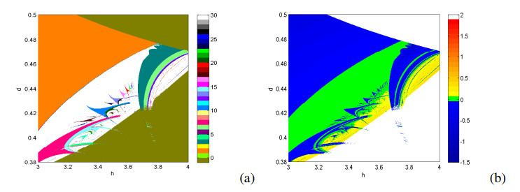
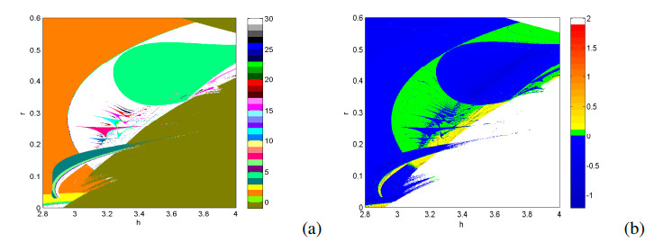
In this paper, we consider a discrete-time SIR epidemic model. Codimension-two bifurcations associated with 1:2, 1:3 and 1:4 strong resonances are analyzed by using a series of affine transformations and bifurcation theory. Numerical simulations are carried out to verify and illustrate these theoretical results. More precisely, two kinds of high-resolution stability phase diagrams are exhibited to describe how the system's complexity unfolds with control parameters varying.
Citation: Xijuan Liu, Peng Liu, Yun Liu. The existence of codimension-two bifurcations in a discrete-time SIR epidemic model[J]. AIMS Mathematics, 2022, 7(3): 3360-3378. doi: 10.3934/math.2022187
In this paper, we consider a discrete-time SIR epidemic model. Codimension-two bifurcations associated with 1:2, 1:3 and 1:4 strong resonances are analyzed by using a series of affine transformations and bifurcation theory. Numerical simulations are carried out to verify and illustrate these theoretical results. More precisely, two kinds of high-resolution stability phase diagrams are exhibited to describe how the system's complexity unfolds with control parameters varying.

| [1] |
D. M. Morens, G. K. Folkers, A. S. Fauci, The challenge of emerging and re-emerging infectious diseases, Nature, 430 (2004), 242–249. doi: 10.1038/nature02759. doi: 10.1038/nature02759

|
| [2] | L. J. S. Allen, Some discrete-time SI, SIR, and SIS epidemic models, Math. Biosci., 124 (1994), 83–105. doi: 10.1016/0025-5564(94)90025-6. |
| [3] |
X. Y. Meng, T. Zhang, The impact of media on the spatiotemporal pattern dynamics of a reaction-diffusion epidemic model, Math. Biosci. Eng., 17 (2020), 4034–4047. doi: 10.3934/mbe.2020223. doi: 10.3934/mbe.2020223
|
| [4] |
Y. Wang, Z. C. Wei, J. D. Cao, Epidemic dynamics of influenza-like diseases spreading in complex networks, Nonlinear Dyn., 101 (2020), 1801–1820. doi: 10.1007/s11071-020-05867-1. doi: 10.1007/s11071-020-05867-1
|
| [5] |
A. Suryanto, I. Darti, On the nonstandard numerical discretization of SIR epidemic model with a saturated incidence rate and vaccination, AIMS Math., 6 (2020), 141–155. doi: 10.3934/math.2021010. doi: 10.3934/math.2021010
|
| [6] |
X. Z. Meng, S. N. Zhao, T. Feng, T. H. Zhang, Dynamics of a novel nonlinear stochastic SIS epidemic with double epidemic hypothesis, J. Math. Anal. Appl., 433 (2016), 227–242. doi: 10.1016/j.jmaa.2015.07.056. doi: 10.1016/j.jmaa.2015.07.056
|
| [7] |
L. Liu, X. F. Luo, L. L. Chang, Vaccination strategies of an SIR pair approximation model with demographics on complex networks, Chaos Solitons Fractals, 104 (2017), 282–290. doi: 10.1016/j.chaos.2017.08.019. doi: 10.1016/j.chaos.2017.08.019
|
| [8] |
B. C. Tian, R. Yuan, Travelling waves for a diffusive SEIR epidemic model with nonlocal reaction and with standard incidences, Nonlinear Anal.: RWA, 37 (2017), 162–181. doi: 10.1016/j.nonrwa.2017.02.007. doi: 10.1016/j.nonrwa.2017.02.007
|
| [9] |
F. Li, X. Meng, X. Wang, Analysis and numerical simulations of a stochastic SEIQR epidemic system with quarantine-adjusted incidence and imperfect vaccination, Comput. Math. Method. M., 2018 (2018), 1–14. doi: 10.1155/2018/7873902. doi: 10.1155/2018/7873902
|
| [10] |
E. Volz, SIR dynamics in random networks with heterogeneous connectivity, J. Math. Biol., 56 (2008), 293–310. doi: 10.1007/s00285-007-0116-4. doi: 10.1007/s00285-007-0116-4
|
| [11] |
T. Harko, F. Lobo, M. K. Mak, Exact analytical solutions of the susceptible-infected-recovered (SIR) epidemic model and of the SIR model with equal death and birth rates, Appl. Math. Comput., 236 (2014), 184–194. doi: 10.1016/j.amc.2014.03.030. doi: 10.1016/j.amc.2014.03.030
|
| [12] |
T. Kuniya, Hopf bifurcation in an age-structured SIR epidemic model, Appl. Math. Lett., 92 (2019), 22–28. doi: 10.1016/j.aml.2018.12.010. doi: 10.1016/j.aml.2018.12.010
|
| [13] |
H. J. Hu, X. F. Zou, Traveling waves of a diffusive SIR epidemic model with general nonlinear incidence and infinitely distributed latency but without demography, Nonlinear Anal.: RWA, 58 (2021), 103224. doi: 10.1016/j.nonrwa.2020.103224. doi: 10.1016/j.nonrwa.2020.103224
|
| [14] |
M. Simon, SIR epidemics with stochastic infectious periods, Stoch. Proc. Appl., 130 (2020), 4252–4274. doi: 10.1016/j.spa.2019.12.003. doi: 10.1016/j.spa.2019.12.003
|
| [15] |
G. W. Luo, Y. L. Zhang, J. H. Xie, Bifurcation sequences of vibroimpact system near a 1:2 strong resonance point, Nonlinear Anal.: RWA, 10 (2009), 1–15. doi: 10.1016/j.nonrwa.2007.08.027. doi: 10.1016/j.nonrwa.2007.08.027
|
| [16] |
L. G. Yuan, Q. G. Yang, Bifurcation, invariant curve and hybrid control in a discrete-time predator-prey model, Appl. Math. Model., 39 (2015), 2345–2362. doi: 10.1016/j.apm.2014.10.040. doi: 10.1016/j.apm.2014.10.040
|
| [17] |
S. G. Ruan, W. D. Wang, Dynamical behavior of an epidemic model with a nonliner incidence rate, J. Differ. Equations, 188 (2003), 135–163. doi: 10.1016/S0022-0396(02)00089-X. doi: 10.1016/S0022-0396(02)00089-X
|
| [18] |
N. Yi, P. Liu, Q. L. Zhang, Bifurcations analysis and tracking control of an epidemic model with nonlinear incidence rate, Appl. Math. Model., 36 (2012), 1678–1693. doi: 10.1016/j.apm.2011.09.020. doi: 10.1016/j.apm.2011.09.020
|
| [19] |
J. L. Ren, L. P. Yu, Codimension-two bifurcation, chaos and control in a discrete-time information diffusion model, J. Nonlinear Sci., 26 (2016), 1895–1931. doi: 10.1007/s00332-016-9323-8. doi: 10.1007/s00332-016-9323-8
|
| [20] |
Z. Y. Hu, Z. D. Teng, L. Zhang, Stability and bifurcation analysis in a discrete SIR epidemic model, Math. Comput. Simulat., 97 (2014), 80–93. doi: 10.1016/j.matcom.2013.08.008. doi: 10.1016/j.matcom.2013.08.008
|
| [21] |
A. A. Berryman, J. A. Millstein, Are ecological systems chaotic$-$And if not, why not, Trends. Ecol. Evol., 4 (1989), 26–28. doi: 10.1016/0169-5347(89)90014-1. doi: 10.1016/0169-5347(89)90014-1
|
| [22] |
M. P. Hassell, H. N. Comins, R. M. May, Spatial strucature and chaos in insect population dynamics, Nature, 353 (1991), 255–258. doi: 10.1038/353255a0. doi: 10.1038/353255a0
|
| [23] | Y. A. Kuznetsov, Elements of applied Bifurcation theory, New York: Springer-Verlag, 2004. doi: 10.1007/978-1-4757-3978-7. |
| [24] |
X. J. Liu, Y. Liu, Codimension-two bifurcation analysis on a discrete Gierer-Meinhardt system, Int. J. Bifurcat. Chaos, 30 (2020), 2050251. doi: 10.1142/S021812742050251X. doi: 10.1142/S021812742050251X
|
| [25] | S. Wiggins, Introduction to applied nonlinear dynamical system and chaos, New York: Springer-Verlag, 2003. |
| [26] |
X. P. Wu, L. C. Wang, Analysis of oscillatory patterns of a discrete-time Rosenzwig-MacArthur model, Int. J. Bifurcat. Chaos, 28 (2018), 1850075. doi: 10.1142/S021812741850075X. doi: 10.1142/S021812741850075X
|
| [27] |
C. W. Chang-Jian, Bifurcation and chaos of a gear-rotor-bearing system lubricated with couple-stress fluid, Nonlinear Dyn., 79 (2015), 749–763. doi: 10.1007/s11071-014-1701-x. doi: 10.1007/s11071-014-1701-x
|
| [28] |
G. C. Layek, N. C. Pati, Organized structures of two bidirectionally coupled logistic maps, Chaos, 29 (2019), 093104. doi: 10.1063/1.5111296. doi: 10.1063/1.5111296
|
| [29] |
X. B. Rao, Y. D. Chu, Y. X. Chang, Dynamics of a cracked rotor system with oil-film force in parameter space, Nonlinear Dyn., 88 (2017), 2347–2357. doi: 10.1007/s11071-017-3381-9. doi: 10.1007/s11071-017-3381-9
|
| [30] |
F. J. Wang, H. J. Cao, Model locking and quaiperiodicity in a discrete-time Chialvo neuron model, Commun. Nonlinear Sci. Numer. Simul., 56 (2018), 481–489. doi: 10.1016/j.cnsns.2017.08.027. doi: 10.1016/j.cnsns.2017.08.027
|
Figures(8)

Xijuan Liu, Peng Liu, Yun Liu. The existence of codimension-two bifurcations in a discrete-time SIR epidemic model[J]. AIMS Mathematics, 2022, 7(3): 3360-3378. doi: 10.3934/math.2022187


 DownLoad: