Intelligent computing based supervised learning for solving nonlinear system of malaria endemic model

Iftikhar Ahmad; Hira Ilyas; Muhammad Asif Zahoor Raja; Tahir Nawaz Cheema; Hasnain Sajid; Kottakkaran Sooppy Nisar; Muhammad Shoaib; Mohammed S. Alqahtani; C Ahamed Saleel; Mohamed Abbas; Iftikhar Ahmad; Hira Ilyas; Muhammad Asif Zahoor Raja; Tahir Nawaz Cheema; Hasnain Sajid; Kottakkaran Sooppy Nisar; Muhammad Shoaib; Mohammed S. Alqahtani; C Ahamed Saleel; Mohamed Abbas

doi:10.3934/math.20221114

AIMS Mathematics

2022, Volume 7, Issue 11: 20341-20369. doi: 10.3934/math.20221114

Previous Article Next Article

Research article Special Issues

Intelligent computing based supervised learning for solving nonlinear system of malaria endemic model

1.
Department of Mathematics, University of Gujrat, Gujrat, 50700, Pakistan
2.
Future Technology Research Center, National Yunlin University of Science and Technology, 123 University Road, Section 3, Douliou, Yunlin 64002, Taiwan, China
3.
Department of Mathematics, College of Arts and Sciences, Wadi Aldawaser, 11991, Prince Sattam bin Abdulaziz University, Saudi Arabia
4.
Department of Mathematics, COMSATS University Islamabad, Attock Campus, Pakistan
5.
Radiological Sciences Department, College of Applied Medical Sciences, King Khalid University, Abha 61421, Saudi Arabia
6.
BioImaging Unit, Space Research Centre, Michael Atiyah Building, University of Leicester, Leicester, LE1 7RH, U.K
7.
Department of Mechanical Engineering, College of Engineering, King Khalid University, Asir-Abha, 61421, Saudi Arabia
8.
Electrical Engineering Department, College of Engineering, King Khalid University, Abha 61421, Saudi Arabia
9.
Electronics and communications Department, College of Engineering, Delta University for Science and Technology, Gamasa 35712, Egypt

Received: 02 June 2022 Revised: 06 August 2022 Accepted: 16 August 2022 Published: 16 September 2022
MSC : 68T07, 92B20

A repeatedly infected person is one of the most important barriers to malaria disease eradication in the population. In this article, the effects of recurring malaria re-infection and decline in the spread dynamics of the disease are investigated through a supervised learning based neural networks model for the system of non-linear ordinary differential equations that explains the mathematical form of the malaria disease model which representing malaria disease spread, is divided into two types of systems: Autonomous and non-autonomous, furthermore, it involves the parameters of interest in terms of Susceptible people, Infectious people, Pseudo recovered people, recovered people prone to re-infection, Susceptible mosquito, Infectious mosquito. The purpose of this work is to discuss the dynamics of malaria spread where the problem is solved with the help of Levenberg-Marquardt artificial neural networks (LMANNs). Moreover, the malaria model reference datasets are created by using the strength of the Adams numerical method to utilize the capability and worth of the solver LMANNs for better prediction and analysis. The generated datasets are arbitrarily used in the Levenberg-Marquardt back-propagation for the testing, training, and validation process for the numerical treatment of the malaria model to update each cycle. On the basis of an evaluation of the accuracy achieved in terms of regression analysis, error histograms, mean square error based merit functions, where the reliable performance, convergence and efficacy of design LMANNs is endorsed through fitness plot, auto-correlation and training state.
- neural networks,
- Levenberg-Marquardt artificial neural networks,
- supervised learning
Citation: Iftikhar Ahmad, Hira Ilyas, Muhammad Asif Zahoor Raja, Tahir Nawaz Cheema, Hasnain Sajid, Kottakkaran Sooppy Nisar, Muhammad Shoaib, Mohammed S. Alqahtani, C Ahamed Saleel, Mohamed Abbas. Intelligent computing based supervised learning for solving nonlinear system of malaria endemic model[J]. AIMS Mathematics, 2022, 7(11): 20341-20369. doi: 10.3934/math.20221114

Related Papers:

Abstract

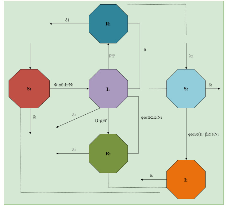
A repeatedly infected person is one of the most important barriers to malaria disease eradication in the population. In this article, the effects of recurring malaria re-infection and decline in the spread dynamics of the disease are investigated through a supervised learning based neural networks model for the system of non-linear ordinary differential equations that explains the mathematical form of the malaria disease model which representing malaria disease spread, is divided into two types of systems: Autonomous and non-autonomous, furthermore, it involves the parameters of interest in terms of Susceptible people, Infectious people, Pseudo recovered people, recovered people prone to re-infection, Susceptible mosquito, Infectious mosquito. The purpose of this work is to discuss the dynamics of malaria spread where the problem is solved with the help of Levenberg-Marquardt artificial neural networks (LMANNs). Moreover, the malaria model reference datasets are created by using the strength of the Adams numerical method to utilize the capability and worth of the solver LMANNs for better prediction and analysis. The generated datasets are arbitrarily used in the Levenberg-Marquardt back-propagation for the testing, training, and validation process for the numerical treatment of the malaria model to update each cycle. On the basis of an evaluation of the accuracy achieved in terms of regression analysis, error histograms, mean square error based merit functions, where the reliable performance, convergence and efficacy of design LMANNs is endorsed through fitness plot, auto-correlation and training state.

References

[1]	World Health Organization. World malaria report 2015. World Health Organization, 2016. http://www.who.int/malaria/visual-refresh/en/
[2]	C. Chiyaka, J. M. Tchuenche, W. Garira, S. Dube, A mathematical analysis of the effects of control strategies on the transmission dynamics of malaria, Appl. Math. Comput., 195 (2008), 641–662. https://doi.org/10.1016/j.amc.2007.05.016 doi: 10.1016/j.amc.2007.05.016
[3]	K. Marsh, Malaria disaster in Africa, Lancet, 352 (1998), 924. https://doi.org/10.1016/S0140-6736(05)61510-3
[4]	World Health Organization, Diet, nutrition, and the prevention of chronic diseases: report of a joint WHO/FAO expert consultation, 916. World Health Organization, 2003. https://apps.who.int/iris/handle/10665/42665
[5]	S. W. Lindsay, W. J. Martens, Malaria in the African highlands: Past, present and future, B. World Health Organ., 76 (1998), 33. https://www.ncbi.nlm.nih.gov/pmc/articles/PMC2305628/
[6]	K. O. Okosun, R. Ouifki, N. Marcus, Optimal control analysis of a malaria disease transmission model that includes treatment and vaccination with waning immunity, Biosystems, 106 (2011), 136–145. https://doi.org/10.1016/j.biosystems.2011.07.006 doi: 10.1016/j.biosystems.2011.07.006
[7]	J. Popovici, L. Pierce-Friedrich, S. Kim, S. Bin, V. Run, D. Lek, er al., Recrudescence, reinfection, or relapse? A more rigorous framework to assess chloroquine efficacy for Plasmodium vivax malaria, J. Infect. Dis., 219 (2019), 315–322. https://doi.org/10.1093/infdis/jiy484
[8]	Ric N. Price, L. von Seidlein, N. Valecha, F. Nosten, J. K. Baird, N. J. White, et al., Global extent of chloroquine-resistant Plasmodium vivax: A systematic review and meta-analysis, Lancet Infect. Dis., 14 (2014), 982–991. https://doi.org/10.1016/S1473-3099(14)70855-2 doi: 10.1016/S1473-3099(14)70855-2
[9]	P. Georgescu, H. Zhang, A Lyapunov functional for a SIRI model with nonlinear incidence of infection and relapse, Appl. Math. Comput., 219 (2013), 8496–8507. https://doi.org/10.1016/j.amc.2013.02.044 doi: 10.1016/j.amc.2013.02.044
[10]	M. Kotepui, F. R. Masangkay, K. U. Kotepui, G, De Jesus Milanez, Misidentification of Plasmodium ovale as Plasmodium vivax malaria by a microscopic method: A meta-analysis of confirmed P. ovale cases, Sci. Rep., 10 (2020), 1–13. https://doi.org/10.1038/s41598-020-78691-7 doi: 10.1038/s41598-020-78691-7
[11]	B. Nadjm, R. H. Behrens, Malaria: An update for physicians, Infect. Dis. Clin. North Am., 26 (2012), 243–259. https://doi.org/10.1016/j.idc.2012.03.010 doi: 10.1016/j.idc.2012.03.010
[12]	R. Anguelov, Y. Dumont, J. Lubuma, Mathematical modeling of sterile insect technology for control of anopheles mosquito, Comput. Math. Appl., 64 (2012), 374–389. https://doi.org/10.1016/j.camwa.2012.02.068 doi: 10.1016/j.camwa.2012.02.068
[13]	M. Ghosh, Mathematical modelling of malaria with treatment, Adv. Appl. Math. Mech., 5 (2013), 857–871. https://doi.org/10.1017/S2070073300001272 doi: 10.1017/S2070073300001272
[14]	S. Olaniyi, O. S. Obabiyi, Qualitative analysis of malaria dynamics with nonlinear incidence function, Appl. Math. Sci. 8 (2014), 3889–3904. http://dx.doi.org/10.12988/ams.2014.45326
[15]	A. L. Mojeeb, J. Li, Analysis of a vector-bias malaria transmission model with application to Mexico, Sudan and Democratic Republic of the Congo, J. Theor. Biol., 464 (2019), 72–84. https://doi.org/10.1016/j.jtbi.2018.12.033 doi: 10.1016/j.jtbi.2018.12.033
[16]	R. M. Anderson, R. M. May, Infectious diseases of humans: dynamics and control, Oxford university press, 1992. ISBN-13: 978-0198540403
[17]	S. Lal, G. P. S. Dhillon, C. S. Aggarwal, Epidemiology and control of malaria, Indian J. Pediatr., 66 (1999), 547–554. https://doi.org/10.1007/BF02727167 doi: 10.1007/BF02727167
[18]	R. Ross, The prevention of malaria, John Murray, 1911. https://doi.org/10.1007/978-0-85729-115-8-12
[19]	A. M. Niger, A. B. Gumel, Mathematical analysis of the role of repeated exposure on malaria transmission dynamics, Differ. Equat. Dyn. Syst., 16 (2008), 251–287. https://doi.org/10.1007/s12591-008-0015-1 doi: 10.1007/s12591-008-0015-1
[20]	J. Li, Y. Zhao, S. Li, Fast and slow dynamics of malaria model with relapse, Math. Biosci., 246 (2013), 94–104. https://doi.org/10.1016/j.mbs.2013.08.004 doi: 10.1016/j.mbs.2013.08.004
[21]	H. Huo, G. Qiu, Stability of a mathematical model of malaria transmission with relapse, Abstr. Appl. Anal., 2014 (2014), Hindawi. https://doi.org/10.1155/2014/289349 doi: 10.1155/2014/289349
[22]	A. Lahrouz, H. El Mahjour, A. Settati, A. Bernoussi, Dynamics and optimal control of a non-linear epidemic model with relapse and curem, Physica A, 496 (2018), 299–317. https://doi.org/10.1016/j.physa.2018.01.007 doi: 10.1016/j.physa.2018.01.007
[23]	L. Liu, J. Wang, X. Liu, Global stability of an SEIR epidemic model with age-dependent latency and relapse, Nonlinear Anal-Real., 24 (2015), 18–35. https://doi.org/10.1016/j.nonrwa.2015.01.001 doi: 10.1016/j.nonrwa.2015.01.001
[24]	A. L. Mojeeb, J. Li. Analysis of a vector-bias malaria transmission model with application to Mexico, Sudan and Democratic Republic of the Congo, J. Theor. Biol., 464 (2019), 72–84. https://doi.org/10.1016/j.jtbi.2018.12.033 doi: 10.1016/j.jtbi.2018.12.033
[25]	M. Ghosh, S. Olaniyi, O. S. Obabiyi, Mathematical analysis of reinfection and relapse in malaria dynamics, Appl. Math. Comput., 373 (2020), 125044. https://doi.org/10.1016/j.amc.2020.125044 doi: 10.1016/j.amc.2020.125044
[26]	H. Zhang, J. Guo, H. Li, Y. Guan, Machine learning for artemisinin resistance in malaria treatment across in vivo-in vitro platforms, Iscience, 25 (2022), 103910. https://doi.org/10.1016/j.isci.2022.103910 doi: 10.1016/j.isci.2022.103910
[27]	R. Islam, Nahiduzzaman, O. F. Goni, A. Sayeed, S. Anower, M. Ahsan, et al., Explainable transformer-based deep learning model for the detection of Malaria Parasites from blood cell images, Sensors, 22 (2022), 4358. https://doi.org/10.3390/s22124358 doi: 10.3390/s22124358
[28]	M. A. Omoloye, A. E. Udokang, A. O. Sanusi, O. K. S. Emiola, Analytical solution of dynamical transmission of Malaria disease model using differential transform method, Int. J. Novel Res. Phys. Chem. Math., 9 (2022), 1–13. https://www.noveltyjournals.com/upload/paper/Analytical%20Solution-27042022-7.pdf
[29]	N. H. Sweilam, Z. N. Mohammed, Numerical treatments for a multi-time delay complex order mathematical model of HIV/AIDS and malaria, Alex. Eng. J., 61 (2022), 10263–10276. https://doi.org/10.1016/j.aej.2022.03.058 doi: 10.1016/j.aej.2022.03.058
[30]	I. Khan, M. A. Z. Raja, M. Shoaib, P. Kumam, H. Alrabaiah, Z. Shah, Design of neural network with Levenberg-Marquardt and Bayesian regularization backpropagation for solving pantograph delay differential equations, IEEE Access, 8 (2020), 137918–137933. https://doi.org/10.1109/ACCESS.2020.3011820 doi: 10.1109/ACCESS.2020.3011820
[31]	A. H. Bukhari, M. Sulaiman, M. A. Z. Raja, S. Islam, M. Shoaib, P. Kumam, Design of a hybrid NAR-RBFs neural network for nonlinear dusty plasma system, Alex. Eng. J., 59 (2020), 3325–3345. https://doi.org/10.1016/j.aej.2020.04.051 doi: 10.1016/j.aej.2020.04.051
[32]	I. Ahmad, H. Ilyas, A. Urooj, M. S. Aslam, M. Shoaib, M. A. Z. Raja, Novel applications of intelligent computing paradigms for the analysis of nonlinear reactive transport model of the fluid in soft tissues and microvessels, Neural Comput. Appl., 31 (2019), 9041–9059. https://doi.org/10.1007/s00521-019-04203-y doi: 10.1007/s00521-019-04203-y
[33]	Z. Shah, M. A. Z. Raja, Y. Chu, W. A. Khan, M. Waqas, M. Shoaih, et al., Design of neural network based intelligent computing for neumerical treatment of unsteady 3D flow of Eyring-Powell magneto-nanofluidic model, J. Mater. Res. Technol., 9 (2020), 14372–14387. https://doi.org/10.1016/j.jmrt.2020.09.098 doi: 10.1016/j.jmrt.2020.09.098
[34]	H. Ilyas, I. Ahmad, M. A. Z. Raja, M. Shoaib, A novel design of Gaussian WaveNets for rotational hybrid nanofluidic flow over a stretching sheet involving thermal radiation, Int. Commun. Heat Mass Transfer, 123 (2021), 105196. https://doi.org/10.1016/j.icheatmasstransfer.2021.105196 doi: 10.1016/j.icheatmasstransfer.2021.105196
[35]	H. Ilyas, I. Ahmad, M. A. Z. Raja, M. B. Tahir, M. Shoaib, Intelligent networks for crosswise stream nanofluidic model with Cu-$H_2$O over porous stretching medium, Int. J. Hydrogen Energ., 46 (2021), 15322–15336. https://doi.org/10.1016/j.ijhydene.2021.02.108 doi: 10.1016/j.ijhydene.2021.02.108
[36]	H. Ilyas, I. Ahmad, M. A. Z. Raja, M. B. Tahir, M. Shoaib, Intelligent computing for the dynamics of fluidic system of electrically conducting Ag/Cu nanoparticles with mixed convection for hydrogen possessions, Int. J. Hydrogen Energ., 46 (2021), 4947–4980. https://doi.org/10.1016/j.ijhydene.2020.11.097 doi: 10.1016/j.ijhydene.2020.11.097
[37]	T. N. Cheema, M. A. Z. Raja, I. Ahmad, S. Naz, H. Ilyas, M. Shoaib, Intelligent computing with Levenberg–Marquardt artificial neural networks for nonlinear system of COVID-19 epidemic model for future generation disease control, Europ. Phys. J. Plus, 135 (2020), 1–35. https://doi.org/10.1140/epjp/s13360-020-00910-x doi: 10.1140/epjp/s13360-020-00910-x
[38]	M. Shoaib, M. A. Z. Raja, M. T. Sabir, A. H. Bukhari, H. Alrabaiah, Z. Shah, A stochastic numerical analysis based on hybrid NAR-RBFs networks nonlinear SITR model for novel COVID-19 dynamics, Comput. Meth. Prog. Bio., 202 (2021), 105973. https://doi.org/10.1016/j.cmpb.2021.105973 doi: 10.1016/j.cmpb.2021.105973
[39]	Z. Sabir, M. A. Z. Raja, J. L. G. Guirao, M. Shoaib, A novel design of fractional Meyer wavelet neural networks with application to the nonlinear singular fractional Lane-Emden systems, Alex. Eng. J., 60 (2021), 2641–2659. https://doi.org/10.1016/j.aej.2021.01.004 doi: 10.1016/j.aej.2021.01.004
[40]	I. Khan, M. A. Z. Raja, M. Shoaib, P. Kumam, H. Alrabaiah, Z. Shah, SCL 802 Fixed Point Laboratory, Center of Excellence in Theoretical and Computational Science (TaCS-CoE), King Mongkut's University of Technology, Thonburi (KMUTT), Bangkok, Thailand Design of neural network with Levenberg-Marquardt and Bayesian regularization backpropagation for solving pantograph delay differential equations, IEEE Access, 8 (2020), 137918–137933. https://doi.org/10.1109/ACCESS.2020.3011820 doi: 10.1109/ACCESS.2020.3011820
[41]	Z. Sabir, D. Baleanu, M. Shoaib, M. A. Z. Raja, Design of stochastic numerical solver for the solution of singular three-point second-order boundary value problems, Neural Comput. Appl., 33 (2021), 2427–2443. https://doi.org/10.1007/s00521-020-05143-8 doi: 10.1007/s00521-020-05143-8
[42]	Z. Sabir, M. Umar, J. L. G. Guirao, M. S. Muhammad A. Z. Raja, Integrated intelligent computing paradigm for nonlinear multi-singular third-order Emden Fowler equation, Neural Comput. Appl., 33 (2021), 3417–3436. https://doi.org/10.1007/s00521-020-05187-w doi: 10.1007/s00521-020-05187-w
[43]	Z. Sabir, M. A. Z. Raja, M. Shoaib, J. F. Gómez Aguilar, FMNEICS: Fractional Meyer neuro-evolution-based intelligent computing solver for doubly singular multi-fractional order Lane Emden system, Comput. Appl. Math., 39 (2020), 1–18. https://doi.org/10.1007/s40314-020-01350-0 doi: 10.1007/s40314-020-01350-0
[44]	D. I. Wallace, B. S. Southworth, X. Shi, J. W. Chipman, A. K. Githeko, A comparison of five malaria transmission models: Benchmark tests and implications for disease control, Malaria J., 13 (2014), 1–16. https://doi.org/10.1186/1475-2875-13-268 doi: 10.1186/1475-2875-13-268
[45]	I. Ahmad, T. N. Cheema, M. A. Z. Raja, S. E. Awan, N. B. Alias, S. Iqbal, et al., A novel application of Lobatto IIIA solver for numerical treatment of mixed convection nanofluidic model, Sci. Rep. 11 (2021), 1–16. https://doi.org/10.1038/s41598-021-83990-8
[46]	M. Shoaib, M. A. Z. Raja, M. T. Sabir, S. Islam, Z. Shah, P. Kumam, et al., Numerical investigation for rotating flow of MHD hybrid nanofluid with thermal radiation over a stretching sheet, Sci. Rep., 10 (2020), 1–15. https://doi.org/10.1038/s41598-020-75254-8 doi: 10.1038/s41598-020-75254-8
[47]	O. Chun1, M. A. Z. Raja, S. Naz, I. Ahmad, R. Akhtar, Y. Ali, et al., Dynamics of inclined magnetic field effects on micropolar Casson fluid with Lobatto IIIA numerical solver, AIP Adv., 10, (2020), 065023. https://doi.org/10.1063/5.0004386
[48]	C. Ouyang1, R. Akhtar, M. A. Z. Raja, M. T. Sabir, M. Awais, M. Shoaib, Numerical treatment with Lobatto IIIA technique for radiative flow of MHD hybrid nanofluid (Al2O3Cu/H2O) over a convectively heated stretchable rotating disk with velocity slip effects, AIP Adv., 10 (2020), 055122. https://doi.org/10.1063/1.5143937 doi: 10.1063/1.5143937
[49]	M. Shoaib, M. A. Z. Raja, M, T, Sabir, M. Awais, S. Islam, Z. Shah, et al., Numerical analysis of 3-D MHD hybrid nanofluid over a rotational disk in presence of thermal radiation with Joule heating and viscous dissipation effects using Lobatto IIIA technique, Alex. Eng. J., 60 (2021), 3605–3619. https://doi.org/10.1016/j.aej.2021.02.015 doi: 10.1016/j.aej.2021.02.015
[50]	M. Awais, M. A. Z. Raja, S. E. Awan, M. Shoaib, H. M. Ali, Heat and mass transfer phenomenon for the dynamics of Casson fluid through porous medium over shrinking wall subject to Lorentz force and heat source/sink, Alex. Eng. J., 60 (2021), 1355–1363. https://doi.org/10.1016/j.aej.2020.10.056 doi: 10.1016/j.aej.2020.10.056

Reader Comments

Your name:*

Email:*
© 2022 the Author(s), licensee AIMS Press. This is an open access article distributed under the terms of the Creative Commons Attribution License (http://creativecommons.org/licenses/by/4.0)