On the numerical solutions for a parabolic system with blow-up

Chien-Hong Cho; Ying-Jung Lu; Chien-Hong Cho; Ying-Jung Lu

doi:10.3934/math.2021683

AIMS Mathematics

2021, Volume 6, Issue 11: 11749-11777. doi: 10.3934/math.2021683

Previous Article Next Article

Research article Special Issues

On the numerical solutions for a parabolic system with blow-up

Chien-Hong Cho ^{1
,
,},
Ying-Jung Lu ²

1.
Department of Applied Mathematics, National Sun Yat-sen University, Kaohsiung 804, Taiwan
2.
Department of Data Application, USI Corporation, Neihu, Taipei 114, Taiwan

Received: 14 January 2021 Accepted: 08 May 2021 Published: 12 August 2021
MSC : 65M12

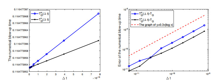
We study the finite difference approximation for axisymmetric solutions of a parabolic system with blow-up. A scheme with adaptive temporal increments is commonly used to compute an approximate blow-up time. There are, however, some limitations to reproduce the blow-up behaviors for such schemes. We thus use an algorithm, in which uniform temporal grids are used, for the computation of the blow-up time and blow-up behaviors. In addition to the convergence of the numerical blow-up time, we also study various blow-up behaviors numerically, including the blow-up set, blow-up rate and blow-up in $ L^\sigma $-norm. Moreover, the relation between blow-up of the exact solution and that of the numerical solution is also analyzed and discussed.
- parabolic system,
- blow-up,
- finite difference method,
- blow-up behavior,
- numerical blow-up
Citation: Chien-Hong Cho, Ying-Jung Lu. On the numerical solutions for a parabolic system with blow-up[J]. AIMS Mathematics, 2021, 6(11): 11749-11777. doi: 10.3934/math.2021683

Related Papers:

Abstract

We study the finite difference approximation for axisymmetric solutions of a parabolic system with blow-up. A scheme with adaptive temporal increments is commonly used to compute an approximate blow-up time. There are, however, some limitations to reproduce the blow-up behaviors for such schemes. We thus use an algorithm, in which uniform temporal grids are used, for the computation of the blow-up time and blow-up behaviors. In addition to the convergence of the numerical blow-up time, we also study various blow-up behaviors numerically, including the blow-up set, blow-up rate and blow-up in $ L^\sigma $-norm. Moreover, the relation between blow-up of the exact solution and that of the numerical solution is also analyzed and discussed.

References

[1]	J. Abia, J. C. López-Marcos, J. Martínez, The Euler method in the numerical integration of reaction-diffusion problems with blow-up, Appl. Numer. Math., 38 (2001), 287–313. doi: 10.1016/S0168-9274(01)00035-6
[2]	C. J. Budd, W. Huang, R. D. Russel, Moving mesh methods for problems with blow-up, J. SIAM J. Sci. Comput., 17 (1996), 305–327. doi: 10.1137/S1064827594272025
[3]	C. J. Budd, O. Koch, L. Taghizadeh, E. B. Weinmüller, Asymptotic properties of the space-time adaptive numerical solution of a nonlinear heat equation, Calcolo, 55 (2018), 43. doi: 10.1007/s10092-018-0286-z
[4]	M. Burger, J. A. Carrillo, M. T. Wolfram, A mixed finite element method for nonlinear diffusion equations, Kinet. Relat. Models, 3 (2010), 59–83. doi: 10.3934/krm.2010.3.59
[5]	G. Caristi, E. Mitidieri, Blow-up estimates of positive solutions of a parabolic system, J. Diff. Eqn., 113 (1994), 265–271. doi: 10.1006/jdeq.1994.1124
[6]	Y. G. Chen, Asymptotic behaviours of blowing-up solutions for finite difference analogue of $u_t = u_xx+u^{1+\alpha}$, J. Fac. Sci. Univ. Tokyo Sect. IA, 33 (1986), 541–574.
[7]	Y. G. Chen, Blow-up solutions to a finite difference analogue of $u_t = u_xx+u^{1+\alpha}$ in $N$-dimensional ball, Hokkaido Math. J., 21 (1992), 447–474. doi: 10.14492/hokmj/1381413684
[8]	M. Chlebík, M. Fila, From critical exponents to blow-up rates for parabolic problems, Rend. Mat. Appl., 19 (1999), 449–470.
[9]	C. H. Cho, On the finite difference approximation for blow-up solutions of the porous medium equation with a source, Appl. Numer. Math., 65 (2013), 1–26. doi: 10.1016/j.apnum.2012.11.001
[10]	C. H. Cho, On the computation of the numerical blow-up time, Japan J. Indust. Appl. Math., 30 (2013), 331–349. doi: 10.1007/s13160-013-0101-9
[11]	C. H. Cho, A numerical algorithm for blow-up problems revisited, Numer. Algor., 75 (2017), 675–697. doi: 10.1007/s11075-016-0216-6
[12]	C. H. Cho, On the computation for blow-up solutions of the nonlinear wave equation, Numerische Mathematik, 138 (2018), 537–556. doi: 10.1007/s00211-017-0919-1
[13]	C. H. Cho, S. Hamada, H. Okamoto, On the finite difference approximation for a parabolic blow-up problem, Japan J. Indust. Appl. Math., 24 (2007), 105–134. doi: 10.1007/BF03167510
[14]	C. H. Cho, H. Okamoto, Further remarks on asymptotic behavior of the numerical solutions of parabolic blow-up problems, Methods Appl. Anal., 14 (2007), 213–226.
[15]	C. H. Cho, H. Okamoto, Finite difference schemes for an axisymmetric nonlinear heat equation with blow-up, Electronic Trans. Numer. Anal., 52 (2020), 391–415. doi: 10.1553/etna_vol52s391
[16]	K. Deng, Blow-up rates for parabolic systems, Z. Angew. Math. Phys., 47 (1996), 132–143. doi: 10.1007/BF00917578
[17]	A. Friedman, B. McLeod, Blow-up of positive solutions of semilinear heat equations, Indiana Uni. Math. J., 34 (1985), 425–447. doi: 10.1512/iumj.1985.34.34025
[18]	M. Fila, P. Souplet, The blow-up rate for semilinear parabolic problems on general domains, NoDEA Nonlinear Differ. Equ. Appl., 8 (2001), 473–480. doi: 10.1007/PL00001459
[19]	A. Friedman, Y. Giga, A single point blow-up for solutions of semilinear parabolic systems, J. Fac. Sci. Univ. Tokyo Sect. IA Math., 34 (1987), 65–79.
[20]	V. A. Galaktionov, S. P. Kurdyumov, A. A. Samarskii, A parabolic system of quasilinear equations I, Differential Equations, 19 (1983), 2123–2140.
[21]	V. A. Galaktionov, S. P. Kurdyumov, A. A. Samarskii, A parabolic system of quasilinear equations II, Differential Equations, 21 (1985), 1544–1559.
[22]	P. Groisman, Totally discrete explicit and semi-implicit Euler methods for a blow-up problem in several space dimensions, Computing, 76 (2006), 325–352. doi: 10.1007/s00607-005-0136-0
[23]	W. Huang, R. D. Russel, Adaptive moving mesh methods, Springer, New York, 2010.
[24]	W. Huang, J. Ma, R. D. Russel, A study of moving mesh PDE methods for numerical simulation of blowup in reaction diffusion equations, J. Comput. Phys., 227 (2008), 6532–6552. doi: 10.1016/j.jcp.2008.03.024
[25]	Y. J. Lu, On a finite difference scheme for blow-up solutions of a semilinear parabolic system, Master's Thesis in National Chung Cheng University, 2018.
[26]	T. Nakagawa, Blowing up of a finite difference solution to $u_t = u_xx+u^2$, Appl. Math. Optim., 2 (1975), 337–350. doi: 10.1007/BF01448176
[27]	T. Nakagawa, T. Ushijima, Numerical analysis of the semi-linear equation of blow-up type, Publications mathématiques et informatique de Rennes, S5 (1976), 1–24.
[28]	T. Nakanishi, N. Saito, Finite element method for radially symmetric solution of a multidimensional semilinear heat equation, Japan J. Indust. Appl. Math., 37 (2020), 165–191. doi: 10.1007/s13160-019-00393-z
[29]	P. Quittner, P. Souplet, Global existence from single-component Lp estimates in a semilinear reaction-diffusion system, Proc. Amer. Math. Soc., 130 (2002), 2719–2724. doi: 10.1090/S0002-9939-02-06453-5
[30]	W. Ren, X. P. Wang, An iterative grid redistribution method for singular problems in multiple dimensions, J. Comput. Phys., 159 (2000), 246–273. doi: 10.1006/jcph.2000.6435
[31]	N. Saito, Error analysis of a conservative finite-element approximation for the Keller-Segel system of chemotaxis, Commun. Pure Appl. Anal., 11 (2012), 339–364. doi: 10.3934/cpaa.2012.11.339
[32]	P. Souplet, Single-point blow-up for a semilinear parabolic system, J. Eur. Math. Soc., 11 (2009), 169–188.
[33]	G. Viglialoro, On the blow-up time of a parabolic system with damping terms, Comptes Rendus de L'Academie Bulgare des Sciences, 67 (2014), 1223–1232.
[34]	F. Weissler, Single point blowup of semilinear initial value problems, J. Diff. Eqn., 55 (1984), 202–224.

Reader Comments

Your name:*

Email:*
© 2021 the Author(s), licensee AIMS Press. This is an open access article distributed under the terms of the Creative Commons Attribution License (http://creativecommons.org/licenses/by/4.0)