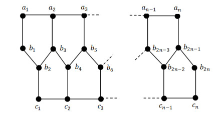
Graph labeling is an assignment of (usually) positive integers to elements of a graph (vertices and/or edges) satisfying certain condition(s). In the last two decades, graph labeling research received much attention from researchers. This articles is about edge irregularity strength for some classes of plane graphs. Edge irregularity strength denoted by $ es(G) $, was introduced by Ahmad et al. in 2014 as a modification of the well known irregularity strength by Chartrand in 1988. In this paper, the exact value of the edge irregularity strength for some clases of plane graphs is determined.
Citation: Ibrahim Tarawneh, Roslan Hasni, Ali Ahmad, Muhammad Ahsan Asim. On the edge irregularity strength for some classes of plane graphs[J]. AIMS Mathematics, 2021, 6(3): 2724-2731. doi: 10.3934/math.2021166
Graph labeling is an assignment of (usually) positive integers to elements of a graph (vertices and/or edges) satisfying certain condition(s). In the last two decades, graph labeling research received much attention from researchers. This articles is about edge irregularity strength for some classes of plane graphs. Edge irregularity strength denoted by $ es(G) $, was introduced by Ahmad et al. in 2014 as a modification of the well known irregularity strength by Chartrand in 1988. In this paper, the exact value of the edge irregularity strength for some clases of plane graphs is determined.

| [1] | A. Ahmad, M. Baca, Y. Bashir, M. K. Siddiqui, Total edge irregularity strength of strong product of two paths, Ars Comb., 106 (2012), 449–459. |
| [2] |
A. Ahmad, M. Baca, M. K. Siddiqui, On edge irregular total labeling of categorical product of two cycles, Theory Comput. Syst., 54 (2014), 1–12. doi: 10.1007/s00224-013-9470-3

|
| [3] | A. Ahmad, O. Al-Mushayt, M. Baca, On edge irregularity strength of graphs, Appl. Math. Comput., 243 (2014), 607–610. |
| [4] | A. Ahmad, M. K. Siddiqui, D. Afzal, On the total edge irregularity strength of zigzag graphs, Australas. J. Comb., 54 (2012), 141–149. |
| [5] | A. Ahmad, Computing the edge irregularity strength of certain unicyclic graphs, submitted. |
| [6] | A. Ahmad, M. Baca, M. F. Nadeem, On the edge irregularity strength of Toeplitz graphs, U.P.B. Sci. Bull., Series A, 78 (2016), 155–162. |
| [7] |
M. Aigner, E. Triesch, Irregular assignments of trees and forests, SIAM J. Discrete Math., 3 (1990), 439–449. doi: 10.1137/0403038
|
| [8] | O. Al-Mushayt, A. Ahmad, M. K. Siddiqui, On the total edge irregularity strength of hexagonal grid graphs, Australas. J. Comb., 53 (2012), 263–271. |
| [9] | O. Al-Mushayt, On the edge irregularity strength of products of certain families with $P_2$, Ars Comb., 137 (2017), 323–334. |
| [10] |
D. Amar, O. Togni, Irregularity strength of trees, Discrete Math., 190 (1998), 15–38. doi: 10.1016/S0012-365X(98)00112-5
|
| [11] |
M. Anholcer, M. Kalkowski, J. Przybylo, A new upper bound for the total vertex irregularity strength of graphs, Discrete Math., 309 (2009), 6316–6317. doi: 10.1016/j.disc.2009.05.023
|
| [12] | M. A. Asim, A. Ali, R. Hasni, Iterative algorithm for computing irregularity strength of complete graph, Ars Comb., 138 (2018), 17–24. |
| [13] | A. Ahmad, M. Baca, M. A. Asim, R. Hasni, Computing edge irregularity strength of complete $m$-ary trees using algorithmic approach, U.P.B. Sci. Bull., Series A, 80 (2018), 145–152. |
| [14] | M. A. Asim, A. Ahmad, R. Hasni, Edge irregular $k$-labeling for several classes of trees, Utilitas Math., 111 (2019), 75–83. |
| [15] |
M. Baca, S. Jendrol, M. Miller, J. Ryan, On irregular total labellings, Discrete Math., 307 (2007), 1378–1388. doi: 10.1016/j.disc.2005.11.075
|
| [16] | M. Baca, M. K. Siddiqui, Total edge irregularity strength of generalized prism, Appl. Math. Comput., 235 (2014), 168–173. |
| [17] | M. Baca, On magic labelings of type $(1, 1, 1)$ for the three classes of plane graphs, Math. Slovaca, 39 (1989), 233–239. |
| [18] |
T. Bohman, D. Kravitz, On the irregularity strength of trees, J. Graph Theory, 45 (2004), 241–254. doi: 10.1002/jgt.10158
|
| [19] | G. Chartrand, M. S. Jacobson, J. Lehel, O. R. Oellermann, S. Ruiz, F. Saba, Irregular networks, Congr. Numer., 64 (1988), 187–192. |
| [20] |
R. J. Faudree, M. S. Jacobson, J. Lehel, R. H. Schelp, Irregular networks, regular graphs and integer matrices with distinct row and column sums, Discrete Math., 76 (1989), 223–240. doi: 10.1016/0012-365X(89)90321-X
|
| [21] |
A. Frieze, R. J. Gould, M. Karonski, F. Pfender, On graph irregularity strength, J. Graph Theory, 41 (2002), 120–137. doi: 10.1002/jgt.10056
|
| [22] | J. A. Gallian, A dynamic survey graph labeling, Electron. J. Comb., 19 (2012), 1–216. |
| [23] |
J. Ivanco, S. Jendrol, Total edge irregularity strength of trees, Discuss. Math. Graph Theory, 26 (2006), 449–456. doi: 10.7151/dmgt.1337
|
| [24] | M. Imran, S. A. Bokhary, A. Ahmad, Total vertex irregularity strength of grid-like-plane graphs, Sci. Int.(Lahore), 27 (2015), 821–828. |
| [25] |
S. Jendrol, J. Mikuf, R. Soták, Total edge irregularity strength of complete graphs and complete bipartite graphs, Discrete Math., 310 (2010), 400–407. doi: 10.1016/j.disc.2009.03.006
|
| [26] |
M. Kalkowski, M. Karonski, F. Pfender, A new upper bound for the irregularity strength of graphs, SIAM J. Discrete Math., 25 (2011), 1319–1321. doi: 10.1137/090774112
|
| [27] |
P. Majerski, J. Przybylo, Total vertex irregularity strength of dense graphs, J. Graph Theory, 76 (2014), 34–41. doi: 10.1002/jgt.21748
|
| [28] |
M. K. M. Haque, Irregular total labellings of generalized Petersen graphs, Theory Comput. Syst., 50 (2012), 537–544. doi: 10.1007/s00224-011-9350-7
|
| [29] |
Nurdin, E. T. Baskoro, A. N. M. Salman, N. N. Gaos, On the total vertex irregularity strength of trees, Discrete Math., 310 (2010), 3043–3048. doi: 10.1016/j.disc.2010.06.041
|
| [30] |
J. Przybylo, Linear bound on the irregularity strength and the total vertex irregularity strength of graphs, SIAM J. Discrete Math., 23 (2009), 511–516. doi: 10.1137/070707385
|
| [31] | I. Tarawneh, R. Hasni, A. Ahmad, On the edge irregularity strength of corona product of graphs with paths, Appl. Math. E-Notes, 16 (2016), 80–87. |
| [32] |
I. Tarawneh, R. Hasni, A. Ahmad, On the edge irregularity strength of corona product of cycle with isolated vertices, AKCE Int. J. Graphs Comb., 13 (2016), 213–217. doi: 10.1016/j.akcej.2016.06.010
|
| [33] | I. Tarawneh, R. Hasni, A. Ahmad, G. C. Lau, On the edge irregularity strength of corona product of graphs with cycle, Discrete Mathematics, Algorithms and Applications, (2020), 2050083. |
| [34] | I. Tarawneh, R. Hasni, M. A. Asim, On the edge irregularity strength of disjoint union of star graph and subdivision of star graph, Ars Comb., 141 (2018), 93–100. |
| [35] | I. Tarawneh, R. Hasni, M. K. Siddiqui, M. A. Asim, On the edge irregularity strength of disjoint union of graphs, Ars Comb., 142 (2019), 239–249. |


Figures(3)

Ibrahim Tarawneh, Roslan Hasni, Ali Ahmad, Muhammad Ahsan Asim. On the edge irregularity strength for some classes of plane graphs[J]. AIMS Mathematics, 2021, 6(3): 2724-2731. doi: 10.3934/math.2021166


 DownLoad: