In this manuscript, we examine the SIR model under convex incidence rate. We first formulate the famous SIR model under the aforesaid incidence rate. Further, we develop some sufficient analysis to examine the dynamical behavior of the model under consideration. We compute the basic reproductive number R0. Also we study the global attractivity results via using Dulac function theory. Further, we also provide some information about the stability of the endemic and disease free equilibria for the considered model. In addition, we use nonstandard finite difference scheme to perform numerical simulation of the considered model via using Matlab. We provide different numerical plots for two different values of contact rate and taking various initial values for compartments involved in the considered model.
Citation: Rahim ud Din, Kamal Shah, Manar A. Alqudah, Thabet Abdeljawad, Fahd Jarad. Mathematical study of SIR epidemic model under convex incidence rate[J]. AIMS Mathematics, 2020, 5(6): 7548-7561. doi: 10.3934/math.2020483
Related Papers:
[1]
Muhammad Altaf Khan, Muhammad Ismail, Saif Ullah, Muhammad Farhan .
Fractional order SIR model with generalized incidence rate. AIMS Mathematics, 2020, 5(3): 1856-1880.
doi: 10.3934/math.2020124
[2]
Shufan Wang, Zhihui Ma, Xiaohua Li, Ting Qi .
A generalized delay-induced SIRS epidemic model with relapse. AIMS Mathematics, 2022, 7(4): 6600-6618.
doi: 10.3934/math.2022368
[3]
Muhammad Altaf Khan, Sajjad Ullah, Saif Ullah, Muhammad Farhan .
Fractional order SEIR model with generalized incidence rate. AIMS Mathematics, 2020, 5(4): 2843-2857.
doi: 10.3934/math.2020182
[4]
Agus Suryanto, Isnani Darti .
On the nonstandard numerical discretization of SIR epidemic model with a saturated incidence rate and vaccination. AIMS Mathematics, 2021, 6(1): 141-155.
doi: 10.3934/math.2021010
[5]
Xiangming Zhao, Jianping Shi .
Dynamic behavior of a stochastic SIR model with nonlinear incidence and recovery rates. AIMS Mathematics, 2023, 8(10): 25037-25059.
doi: 10.3934/math.20231278
[6]
Ahmed Alshehri, Miled El Hajji .
Mathematical study for Zika virus transmission with general incidence rate. AIMS Mathematics, 2022, 7(4): 7117-7142.
doi: 10.3934/math.2022397
[7]
Butsayapat Chaihao, Sujin Khomrutai .
Extinction and permanence of a general non-autonomous discrete-time SIRS epidemic model. AIMS Mathematics, 2023, 8(4): 9624-9646.
doi: 10.3934/math.2023486
[8]
Shenghu Xu, Xiaojuan Li .
Global behavior of solutions to an SI epidemic model with nonlinear diffusion in heterogeneous environment. AIMS Mathematics, 2022, 7(4): 6779-6791.
doi: 10.3934/math.2022377
[9]
Mahmoud A. Ibrahim .
Threshold dynamics in a periodic epidemic model with imperfect quarantine, isolation and vaccination. AIMS Mathematics, 2024, 9(8): 21972-22001.
doi: 10.3934/math.20241068
[10]
Ishtiaq Ali, Sami Ullah Khan .
Dynamics and simulations of stochastic COVID-19 epidemic model using Legendre spectral collocation method. AIMS Mathematics, 2023, 8(2): 4220-4236.
doi: 10.3934/math.2023210
Abstract
In this manuscript, we examine the SIR model under convex incidence rate. We first formulate the famous SIR model under the aforesaid incidence rate. Further, we develop some sufficient analysis to examine the dynamical behavior of the model under consideration. We compute the basic reproductive number R0. Also we study the global attractivity results via using Dulac function theory. Further, we also provide some information about the stability of the endemic and disease free equilibria for the considered model. In addition, we use nonstandard finite difference scheme to perform numerical simulation of the considered model via using Matlab. We provide different numerical plots for two different values of contact rate and taking various initial values for compartments involved in the considered model.
1.
Introduction
Infectious diseases are spread by pathogenic microorganisms. These diseases can transmit from one person to another or from animals or birds. But with all the advancement in medicine to control the disease, it is still major threats for the population. Major causes of infectious disease are changing in human behaviors, use of antibiotic drugs and larger and denser cities. With the advancement of science and technology, the transmission and how to control it in society are hot areas of research for the last many decades. To control and predict for future planing, one of the powerful tool of mathematics is known as differential equations. By differential and difference equations, we can convert a physical or biological phenomenon to mathematical equations. The analysis and investigation of equations formed from biological or physical phenomenon give interesting and fruitful information about the process of how to control and predict future planing. This conversion of physical or biological process to mathematical equations is called mathematical modeling. Mathematical models for the infectious diseases are the major tools to study the process through which diseases spread in a population. In this regard large numbers of mathematical models were formulated in past. We refer few as [1,2,3]. The idea of mathematical model of infectious disease was provided by Mckendrick and Kermack [4] in 1927. The aforementioned scientists described the interaction between susceptible, infected and recovered individual in a community by a simple model known as SIR. An updated SIR model [5] is
dSdt=B−ηS−βSI,dIdt=βSI−γI−ηI,dRdt=γI−ηR,
(1.1)
where N∗=S(t)+I(t)+R(t), is the total population, S denotes the population of susceptible, while I for infected population and R for recovered individuals. Further, death rate and birth rate are represented by η and B respectively. Also infectious rates, denoted by γ and β, are used for contact and removal rate respectively. The aforementioned model is updated to various forms and the idea of SIR model numerous models of infectious disease is formed in literature. The number of diseases increases with the passage of time. Particularly those diseases which are fatal and transferable from one person to another. In order to get control over such fatal diseases, various methods were adopted by scientists. The mathematicians have an important contribution in this regard and their role cannot be denied. They used different models called epidemiological models. In SIR model the total population is deviled into three compartments which are, the susceptible compartment consists of those people who doe not affected by any disease. The infected compartment consists of those peoples who are suffering from disease while the recovered compartment consists of those people who get rid of the diseases and become healthy and sound via proper cure and remedy.
Here, we remark that it is important to know how the disease transmits from an infected person to a healthy one. The rate at which this transmission takes place is called contact rate. According to law of mass action this transmission will take place when a proportional quantity of the healthy persons comes into the contact of infected population. From investigation of various mathematical models, one can find a basic function known as incident rate. With the help of this term, we can identify or diagnose the nature of the diseases. Various incidence rates for the transmission of disease have been studied in literature. For instance, Capasso and Serio [6] in 1978 defined a saturated type incidence rate to investigate the infection between infected and susceptible individuals. They concluded that such effect occurred either due to the overcrowding of infected people or some prevention measure taken by the susceptible people or both. The transmission mechanism of disease in community occur by term rate which is a mathematical function known as incidence rate. The mentioned function is also called the force of infection and it is important in SIR, QSIR, SEIR, models. It depends on the susceptible and infected compartment of the population in most cases. Korobeinikov [7,8] investigated the world-wide properties of an SEIR model by universal non-linear incident rate. He calculated numerous conditions using Lyapunov direct method in terms of incident rate, which proof global asymptotically stable state under positive components such as endemic equilibrium. These conditions of the form of f(S,I)=Sg(I), are affirmed by incidence rates where S,I are susceptible and infected population respectively, and g(I) represents a concave downward function. In the present characterizations, some familiar incidence rates are used like g is saturating or linear (principle of mass action). In this case g is not convex like incidence rates. A light assumption on g is practiced in besides all these convex functions are still in rule. Incident rate have been studied by many researchers in various articles like [9,10,11]. Further complex dynamic has also been studied in epidemiological models with different incidence rate, e.g the limit cycle. Moreover, existence of equilibrium and some other kinds of bifurcations has been calculated, like Saddle-node, Hopf, homo-clinic, also Bagdanov-Takens bifurcation are involved [12] and references therein. One of the best and suitable rate is called convex incidence rate which has been rarely considered in literature in few paper [13,14]. induced by the mentioned work, in this paper, we consider convex incidence rate instead of aforementioned rate to investigate the SIR model (1.1) in new Scenario. Convex incidence rate shows the psychological consequences determine sever diseases in the population, where the infected number is going to increase. By studding the mathematical dynamic of the model and calculating the endemic and the disease-free equilibrium points, we investigate that the count of infected persons approaches to zero as the time develop or disease persevere. This work suggests that convex contact rate bearing the shape
f(S,I)=MIS(1+γI),
(1.2)
which is parallel related to infectious compartment I(t), whenever it increases or decreases when I(t) increases or decreases and M is a proportionality constant. It equates with the growth rate of the disease due to two exposures over a small period of time. The individual contacts precede to infection under the range MIS. On the other hand, the new infected person originates from double exposures at the rate γMI2S. On the other side, incidence rate (1.2) is a related to the stableness properties of the epidemic model also. We investigate the updated model under the convex incidence rate and bring out a global analysis consisting of stability analysis, global and local attractively and numerical simulation. For further detail about mathematical models, we refer some valuable work as [15,16,17,18,19,20]. We use nonstandard finite difference method for numerical simulation, that used in [21,22].
2.
Model formulation
Here, we construct our model. For this purpose, we divide the host populations into three compartments as described earlier in the introduction under the given force function in (1.2) as
For the above System (2.1), we have the following initial data
S(0)=S0>0,I(0)=I0≥0,R(0)=R0≥0.
Firstly, we denote the biological meaning by S(t) the susceptible component, the infected component by I(t) and the recovered components by R(t). The considered model is defined in the first octant of R3. Further, we assume that equilibrium exists. To calculate the set of positive equilibrium
B−ηS−MIS(1+γI)+αR=0MIS(1+γI)−(μ+η)I=0μI−(α+η)R=0.
(2.2)
From (2.2), we have
B−μ−(B+μ)M(1+γI)−MI(B+μ)M(1+γI)(1+γI)+αBμ+αI=0
B(M(1+γI))−μ(B+μ)−MI(B+μ)(1+γI)+(MαIμ+γ)(1+γI)=0
Mα(γμ+γ−(B+μ))I2+M(Bγ−(β+μ)+Bαμ+γ)I+BM−μ(β+μ)=0.
(2.3)
The basic reproduction number is defined as
R0=MBμ(B+μ).
(2.4)
From model (2.3), we have the following:
(i) System (2.1) does not have positive equilibrium if R0<1;
(ii) System (2.1) possesses a unique nontrivial positive-equilibrium points (S∗,I∗,R∗), if R0>1 and given by
In order to study the dynamic of model (2.1), we provide the following result.
Lemma 3.1.System (2.1) has invariant sub manifold of subspace N∗(t)=Bη which is attracting in the first octant.
Proof. Assume that N∗(t)=S(t)+I(t)+R(t). By addition of system equations (2.1), we get
dN∗dt=B−η.
(3.1)
Clearly, the solution of system (2.1) is N∗(t)=B/η, and the general solution if N∗(t0)≥0, is
N∗(t)=1η[B−(B−dN∗(t0))et0−t)].
Thus
limt→∞N∗(t)=Bη.
(3.2)
This shows that the plane defined by N∗(t)=B/η contains limit set of system (2.1). Therefore, we will confine our self to the following reduced system.
Lemma 3.1 suggests that system (2.1) has no periodic orbits. This claim is given by he following result.
Theorem 3.2.There are no nontrivial periodic orbits for system (2.1).
Proof. Firstly, for system(2.1), we assume a Dulac function as
D(I,R)=1MI(1+γI).
(3.4)
We have
∂(DP)∂I+∂(DQ)∂R=−1−(B+η)−η+ααI(1+γI)<0.
To elaborate the properties of the endemic and the disease free equilibrium points E∗ and E0 respectively, we re-scale system (2.1) by
χ=Mη+αI,y=Mα+ηR,τ=(α+η)t.
After this, we have
dχdτ=χ(C−χ−y)(pχ+1)−mχ,dydτ=qχ−y,
(3.5)
where
q=Bη+α,C=Bkη(η+α),m=B+ηα+η,p=α(d+α)2K2.
Note that if m−C<0, then the only absolute stability (χ∗,y∗) of system (3.5) will be the locally stability E∗ of the model (2.1) and the trivial stability (0,0) of the proposed model (3.5) will be disease free equilibrium E0 of model (2.1), where
Next, we find the topological type and stability of (0,0). For the system (3.5) at (0,0),. The Jacobian matrix reads
Q0=(C−m0q−1).
(3.6)
If the condition C−m=0 is satisfied, then a small neighborhood N0 exists about (0,0) and the mathematical behavior of model (3.5) becomes topologically equal to the following system
dχdτ=χ2+2χy+O((χ,y)2)dydτ=qχ−y.
(3.7)
Perko [23] and Zhang et al. [24] concluded that for system (3.7) has a saddle-node (0,0).
Keeping in mind the above results, we can write the following theorem.
Theorem 3.3.The trivial equilibrium point of t system (2.1) possess the following properties.
(i) Hyperbolic saddle, If m<C.
(ii) Saddle node, If m=C.
(iii) Stable hyperbolic node, If m>C.
Proof. If m−A<C, then the discussion is about the topological type and stability. The Jacobian matrix at (χ∗,y∗) of Eq (3.7) is
M1=(2(pC−q−1)χ∗−3pC(1+q)x∗2+C−m−χ∗(pχ∗+1)q−1),
(3.8)
This implies that
det(M1)=3pC(1+q)χ∗2−2(pC−q−1)χ+m−C.
To determine the sign of det(M1), we can calculate S1 as
S1=3p(1+q)χ∗2−2(pC−q−1)χ+m−C.
(3.9)
Assuming H=1+q and replacing in Eq (3.9), we have
S1=3pHχ∗2−2(pC−H)χ+m−C.
(3.10)
From the quadratic equation in (3.10) has the form
3pHχ∗2+2(H−pC)χ∗−C+m=0,
(3.11)
from which we can find out that
χ∗2=(C−m)−2(H−pC)χ∗3pH.
(3.12)
Substituting in Eq (3.10), one has
S1=(pC−H)χ∗+2(C−m).
(3.13)
From Eq (3.11), we obtain
χ∗=(pC−H)+√(H−pC)2−4pH(m−C)2pH.
(3.14)
Now, substituting Eq (3.14) in Eq (3.13), the following can be extracted.
S1=(pC−H)2+Δ12pH+2(C−m)whereΔ1=√(H−pC)2−pA(m−C)H.
Hence, S1>0, if C−m>0. This implies that determinant of (χ∗,y∗) is a node and det(M1)>0.
Furthermore, we can obtain the following results related to the equilibrium of (χ∗,y∗).
Theorem 3.4.For system (2.1), there is a unique local stable node (χ∗,y∗), when m−C<0.
Proof. To determine the equilibrium of (χ∗,y∗), we need to find tr(M1). Since
M1=(2(pC−q−1)χ∗−3pA(1+q)χ∗2+C−m−χ∗(1+pχ∗)q−1),
(3.15)
tr(M1)=2(pC−q−1)χ∗−3pC(1+q)χ∗2+C−m−1.
Now,
S2=2(pC−q−1)χ∗−3pC(1+q)χ∗2+C−m−1.
(3.16)
Computing χ∗2 from Eq (3.11) and putting in Eq (3.16), we get
It can be clearly seen that B1C+B2>0, when m−C<0. Now let
Ψ=pHχ∗2+(H−pC)χ∗−C+m.
Hence,
(D1C+D2)2Ψ=QS2+S3,
where Q denotes the polynomial of χ∗ and
S3=(p(2+3C)+3H)2C2+4H2−4CH(p(2+3C)+H)(m−C).
(3.17)
If we consider that S2=0 and Ψ=0, we can obviously observe that S3=0. Besides, if m−C<0, then S3>0. In addition, for all non-negative values of C,q, p and S2≠0. Nevertheless, tr(M1)≠0. So m−C<0 which shows that (χ∗,y∗) does not effect endemic as well as trivial equilibrium. We Take p,C,q, and m are unity, then χ∗=√2,y=√2,tr(M1)=−6.0883. The continuity of tr(M1) on the following constant, for m−C<0tr(M1)<0. This completes our proof.
The next theorem concludes the results for the mathematical analysis of the original system (2.1) can be established.
Theorem 3.5.From R0 defined in (2.4), we have
(i) System (2.1) has a unique disease-free equilibrium E0=(Bη,0), if R0<1, which shows global attraction of the system (2.1) in the first octant.
(ii) System (2.1) has a unique disease-free equilibrium E0=(Bη,0)R0=1, and draws all orbits under the interior of first octant;
(iii) System (2.1) has two equilibria when R0>1, one is the endemic equilibrium and the other is E∗=(S∗,I∗,R∗) withdisease-free equilibrium at E0=(Bη,0). The endemic equilibrium E∗ has a global attractor within the interior of first octant.
4.
Global stability
Global stability means that any trajectories finally tend to the attractor of the system, regardless of initial conditions.
Here, we used Lyapunov function to study global stability at the disease free equilibrium point by the following theorem.
Theorem 4.1.The disease free equilibrium of the system (2.1) is globally asymptotically stable if R0<1.
Proof. We prove the result by constructing a Lyapunov function.
ℓ=c1(S0−S(t))+c2I(t),
(4.1)
such that the constants c1and c2 are determined later. Differentiating (4.1) with respect to t, to get
Hence, the model (2.1) is "stable globally asymptotically", with R0<1.
5.
Numerical results and conclusions
In this section, to perform numerical simulation for the proposed model under convex contact rate, we use the following values.
Since biological models are often described by ordinary or partial differential equations. Therefore, for their numerical simulation various methods have been used for converting continuous models to discrete counterparts by applying standard difference methods like, RK4, Euler, etc. But in most cases the aforementioned methods suffer from numerical instability. The said instability was removed in 1989 by Mickens. He introduced a more reliable numerical scheme called non standard finite difference scheme (NSFDS). The mentioned method preserves main properties of the differential counterparts, such as positivity, monotonicity, periodicity, stability and some other invariants including energy and geometrical shapes. Hence, this method has been used as a powerful tool for numerical simulation of many models of biology (see for details [25]). Hence, we use NSFDS for the numerical simulation of the proposed model using Matlab.
The model has only one disease free equilibrium point which has been developed in previous sections. From Figures 1–3, the asymptotic stability of equilibrium is obvious. Further, from Figure 1, we see that taking various initial population of susceptible class, the number of susceptible individuals decreases sharply during the first 50 days and then become stable. When the population of susceptible individual increases, the decay gets faster and hence become first stable as compared to the least initial value of S. From Figures 2 and 3, we see that the rate of recovered individuals are faster than the rate of infected individuals by taking different initial values of I and R, respectively. From Figure 1, we see that nearly 80 days after, the susceptible population becomes stable and hence many individuals have recovered at that time from the infected individuals taking the numerical values given in Table 1. In Figures 1–3 we take γ=0.0009. Now in Figures 4–6, we take the same initial population and take γ=0.00045. We can observe that the decrease in susceptible population is sharply fastest as in Figure 4 compared to Figure 1. Similarly, the increase in infected and in recovered population is also fastest at the lower value of γ as shown in Figures 5 and 6 as compared to Figures 2 and 3 respectively. It means that contact rate is important and has the ability to produce effects on the dynamics of transmission of the disease.
Table 1.
The physical description of the parameters with numerical values.
Parameters
physical description
Numerical value
S0
Initial susceptible population
180,170,160,150
I0
Initial infected Population
50,55,40,60
R0
Initial Population which is recovered from disease
20,30,40,50
B
Total population recruitment rate at in any time t
We have successfully established a global analysis of SIR model under convex incidence rate. We have also provided appropriate information that involve convex incidence rate and its effect on the dynamics of the model and transmission of disease. Further, the theoretical results have also enriched by suitable numerical simulation by using NSFDS, which is more powerful than usual RK4 and Euler method. We conclude that taking convex incidence rate, from the presented analysis we conclude that convex incidence rate shows the psychological consequences determine sever diseases in the population, where the infected number is going to increase. In addition, the use of numerical simulations with this kind of models can be specially used for future planning of public health policies how to control the serious diseases like influenza, malaria, salmonella, cholera, whooping cough, and measles in a community.
Acknowledgments
This research was funded by the Deanship of Scientific Research at Princess Nourah bint Abdulrahman University through the Fast- track Research Funding Program.
Conflict of interest
The authors declare that they have no conflict of interest.
References
[1]
A. V. Kamyad, R. Akbari, A. A. Heydari, et al. Mathematical modeling of transmission dynamics and optimal control of vaccination and treatment for hepatitis B virus, Comput. Math. Methods Medecines, 2014 (2014), 15.
[2]
B. Shulgin, L. Stone, Z. Agur, Pulse vaccination strategy in SIR epidemic model, Bulletin Math. Biology, 60 (1988), 1123-1148.
[3]
G. Zaman, Y. H. Kang, I. H. Jung, Stability analysis and optimal vaccination of SIR epidemic model, Bio. System, 93 (2008), 240-249.
[4]
W. O. Kermack, A. G. McKendrick, A contribution to the mathematical theory of epidemics, Royal Society, 115 (1927), 700-721.
[5]
T. Harko, F. S. N. Lobo, M. K. Mak, Exact analytical solutions of the Susceptible-InfectedRecovered (SIR) epidemic model and of the SIR model with equal death and birth rates, Appl. Math. Comput., 236 (2014), 184-194.
[6]
M. E. Alexander, S. M. Moghadas, Periodicity in an epidemic model with a generalized non-linear incidence, Math. Biosci., 189 (2004), 75-96.
[7]
V. Capasso, G. Serio, A generalization of the Kermack-Mckendrick deterministic epidemic model, Math. Biosci., 43 (1978), 43-61.
[8]
A. Korobeinikov, Lyapunov functions and global stability for SIR and SIRS epidemiological models with non-linear transmission, Bulletin Math. Biology 68 (2006), 615-626.
[9]
A. Korobeinikov, Global properties of infectious disease models with nonlinear incidence, Bulletin Math. Biology, 69 (2007), 1871-1886.
[10]
W. R. Derrick, P. van den Driessche, A diseases transmission model in a nonconstant population, J. Math. Biology, 31 (1993), 490-512.
[11]
W. M Liu, H. W. Hethcote, S. A Levin, Dynamical behavior of epidemiological models with nonlinear incidence rate, J. Math. Biology, 25 (1987), 359-380.
[12]
W. M. Liu, S. A. Levin, Y. Iwasa, Influence of nonlinear incident rates upon the behavior of SIRS epidemiological models, J. Math. Biology, 23 (1986), 187-204.
[13]
W. Wang, S. Ruan, Simulating the SARS outbreak in Beijing with limited data, J. Theor. Biology, 227 (2004), 369-379.
[14]
S. Jana, S. K. Nandi, T. K. Kar, Complex dynamics of an SIR epidemic model with saturated incidence rate and treatment, Acta Biotheoretica, 64 (2016), 65-84.
[15]
G. Rahman, K. Shah, F. Haq, et al. Host vector dynamics of pine wilt disease model with convex incidence rate, Chaos, Solitons & Fractals, 113 (2018), 31-39.
[16]
A. B. Gumel, Modelling strategies for controlling SARS out breaks, Proc. R. Soc. Lond. B., 271 (2004), 2223-2232.
[17]
H. W. Hethcote, The mathematics of infectious disease, SIAM Review, 42 (2000), 599-653.
[18]
H. W. Hethcote, S. A. Levin, Periodicity in epidemiological models, Appl. Math. Ecol. Springer, Berlin, Heidelberg, 1989.
[19]
H. W. Hethcote, P. Van den Driessche, Some epidemiological models with nonlinear incidence, J. Math. Biology 29 (1991), 271-287.
[20]
G. M. leung, The impact of community psychological response on outbreak control for severe acute respiratory syndrome in Hong Kong, J. Epidemiol. Commun. Health, 57 (2003), 857-863.
[21]
S. Ruan, W. Wang, Dynamical behavior of an epidemic model with a nonlinear incidence rate, J. Differential Equations, 188 (2003), 135-369.
[22]
A. R. Fathalla, M. N. Anwar, Qualitative analysis of delayed SIR epidemic model with a saturated incidence rate, Int. J. Diff. Equs., 2012 (2012), 13.
[23]
L. Perko, Differential Equations and Dynamical Systems, Springer-Verlag, New York, 1996.
[24]
Z. Zhang, Qualitative theory of differential equations, Providence, American Mathematical Society, 1992.
[25]
R. E. Mickens, Exact solutions to a finite-difference model of a nonlinear reaction-advection equation: Implications for numerical analysis, J. Differ. Equ. Appl., 9 (2003), 995-1006.
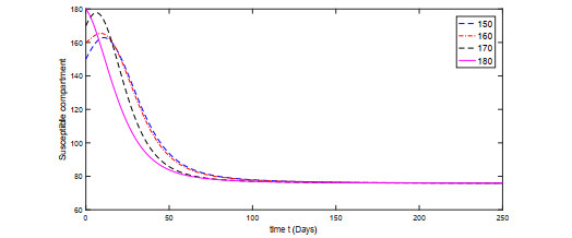
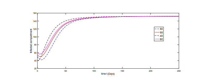
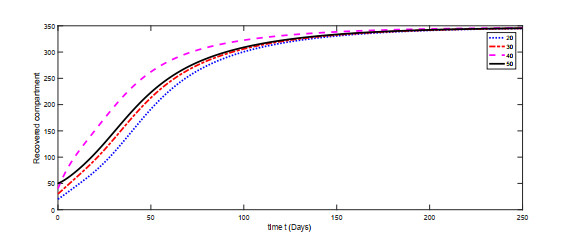
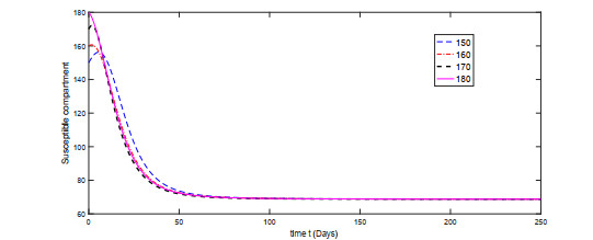
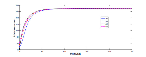
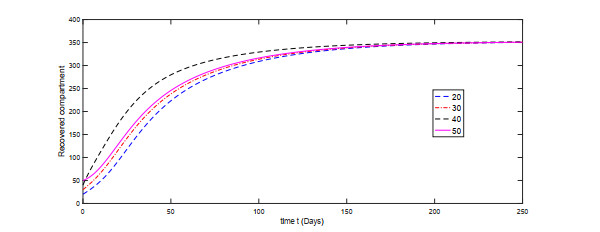
This article has been cited by:
1.
Suganya Govindaraj, Senthamarai Rathinam,
Mathematical modeling and analysis of the effect of the rugose spiraling whitefly on coconut trees,
2022,
7,
2473-6988,
13053,
10.3934/math.2022722
Rahim ud Din, Kamal Shah, Manar A. Alqudah, Thabet Abdeljawad, Fahd Jarad. Mathematical study of SIR epidemic model under convex incidence rate[J]. AIMS Mathematics, 2020, 5(6): 7548-7561. doi: 10.3934/math.2020483