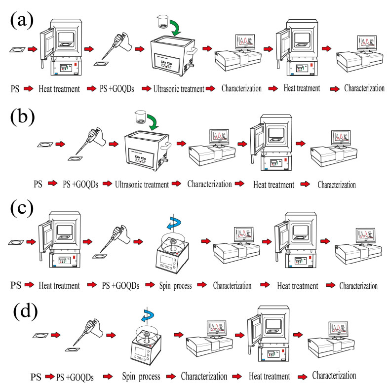
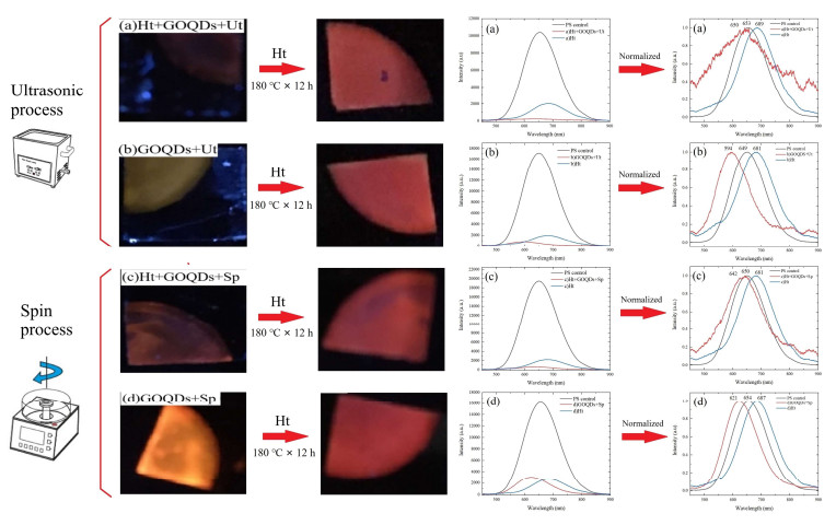
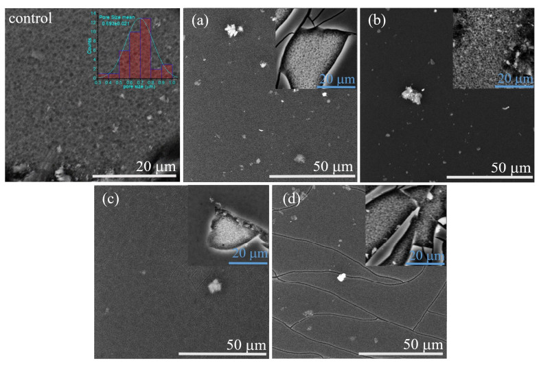
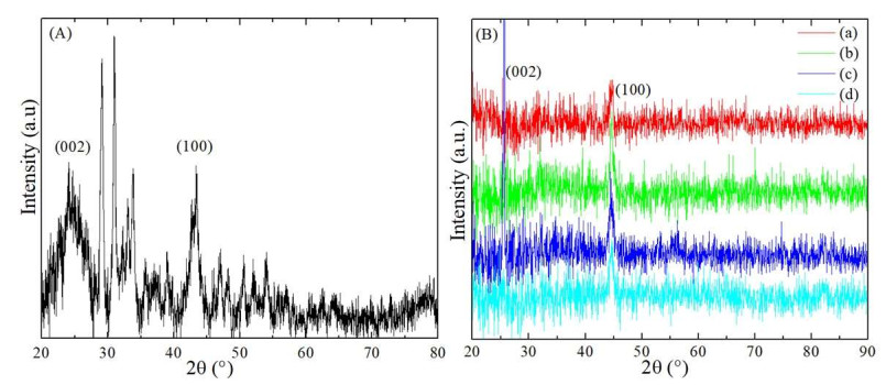
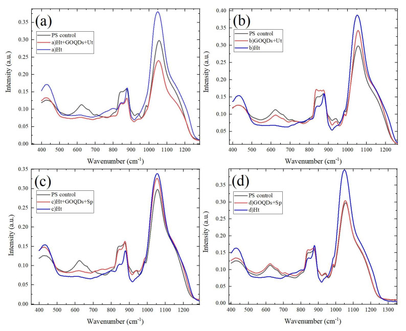
In this work, the luminescent emission control from porous silicon (PS) decorated with graphene oxide quantum dots (GOQDs) was analyzed. The samples obtained showed a 95 nm range of variation in which the luminescent emission can be controlled. Based on the results obtained from the PS samples decorated with GOQDs, the emission can be selected in a range from blue to red. Fourier transform infrared (FTIR) spectroscopy showed evidence of bond formation between PS and GOQDs. These changes can be related to the changes in luminescent emission. Photoluminescence analysis showed that the main PS emission can be selected in a 90 nm range with the introduction of GOQDs. Scanning electron microscopy (SEM) images and energy dispersive spectroscopy (EDS) spectra demonstrated the introduction of GOQDs in the PS. X-ray diffraction patterns also confirmed the presence of GOQDs on the surface of PS. In this study, different methodologies to control the luminescent emission were applied, and the results show that PS samples decorated with GOQDs showing blue, orange, and red luminescence can be obtained. The samples obtained can be applied to the development of electroluminescence devices, photodetectors, and biosensors.
Citation: Francisco Severiano Carrillo, Orlando Zaca Moran, Fernando Díaz Monge, Alejandro Rodríguez Juárez. Luminescence modification of porous silicon decorated with GOQDs synthesized by green chemistry[J]. AIMS Materials Science, 2025, 12(1): 55-67. doi: 10.3934/matersci.2025005
In this work, the luminescent emission control from porous silicon (PS) decorated with graphene oxide quantum dots (GOQDs) was analyzed. The samples obtained showed a 95 nm range of variation in which the luminescent emission can be controlled. Based on the results obtained from the PS samples decorated with GOQDs, the emission can be selected in a range from blue to red. Fourier transform infrared (FTIR) spectroscopy showed evidence of bond formation between PS and GOQDs. These changes can be related to the changes in luminescent emission. Photoluminescence analysis showed that the main PS emission can be selected in a 90 nm range with the introduction of GOQDs. Scanning electron microscopy (SEM) images and energy dispersive spectroscopy (EDS) spectra demonstrated the introduction of GOQDs in the PS. X-ray diffraction patterns also confirmed the presence of GOQDs on the surface of PS. In this study, different methodologies to control the luminescent emission were applied, and the results show that PS samples decorated with GOQDs showing blue, orange, and red luminescence can be obtained. The samples obtained can be applied to the development of electroluminescence devices, photodetectors, and biosensors.

| [1] |
Vercauteren R, Leprince A, Mahillon J, et al. (2021) Porous silicon biosensor for the detection of bacteria through their lysate. Biosensors 11: 27. https://doi.org/10.3390/bios11020027 doi: 10.3390/bios11020027

|
| [2] |
Gör Bölen M, Karacali T (2020) A novel proton-exchange porous silicon membrane production method for μDMFCs. Turk J Chem 44: 1216–1226. https://doi.org/10.3906/kim-2002-32 doi: 10.3906/kim-2002-32
|
| [3] |
Fauchet PM (1998) The integration of nanoscale porous silicon light emitters: materials science, properties, and integration with electronic circuitry. J Lumin 80: 53–64. https://doi.org/10.1016/S0022-2313(98)00070-2 doi: 10.1016/S0022-2313(98)00070-2
|
| [4] |
Robbiano V, Paternò GM, La Mattina AA, et al. (2018) Room-temperature low-threshold lasing from monolithically integrated nanostructured porous silicon hybrid microcavities. ACS Nano 12: 4536–4544. https://doi.org/10.1021/acsnano.8b00875 doi: 10.1021/acsnano.8b00875
|
| [5] |
Riikonen J, Salomäki M, van Wonderen J, et al. (2012) Surface chemistry, reactivity, and pore structure of porous silicon oxidized by various methods. Langmuir 28: 10573–10583. https://doi.org/10.1021/la301642w doi: 10.1021/la301642w
|
| [6] |
Chen Z, Wang M, Fadhil AA, et al. (2021) Preparation, characterization, and corrosion inhibition performance of graphene oxide quantum dots for Q235 steel in 1 M hydrochloric acid solution. Colloids Surf A Physicochem Eng 627: 127209. https://doi.org/10.1016/j.colsurfa.2021.127209 doi: 10.1016/j.colsurfa.2021.127209
|
| [7] |
Xiao X, Zhang Y, Zho L, et al. (2022) Photoluminescence and fluorescence quenching of graphene oxide: A review. Nanomaterials 12: 2444. https://doi.org/10.3390/nano12142444 doi: 10.3390/nano12142444
|
| [8] |
Zhang J, Zhang X, Bi S (2022) Two-dimensional quantum dot-based electrochemical biosensors. Biosensors 12: 254. https://doi.org/10.3390/bios12040254 doi: 10.3390/bios12040254
|
| [9] |
Hossain MA, Islam S (2013) Synthesis of carbon nanoparticles from kerosene and their characterization by SEM/EDX, XRD and FTIR. J Nanosci Nanotechnol 1: 52–56. https://doi.org/10.11648/j.nano.20130102.12 doi: 10.11648/j.nano.20130102.12
|
| [10] |
Huang S, Yang E, Liu Y, et al. (2018) Low-temperature rapid synthesis of nitrogen and phosphorusdual-doped carbon dots for multicolor cellular imaging and hemoglobin probing in human blood. Sens Actuators B Chem 265: 326–334. https://doi.org/10.1016/j.snb.2018.03.056 doi: 10.1016/j.snb.2018.03.056
|
| [11] |
Kurniawan D, Chen YY, Sharma N, et al. (2022) Graphene quantum dot-enabled nanocomposites as luminescence and surface-enhanced Raman scattering biosensors. Chemosensors 2022: 10. https://doi.org/10.3390/chemosensors10120498 doi: 10.3390/chemosensors10120498
|
| [12] |
Xu Q, Gong Y, Zhang Z, et al. (2019) Preparation of graphene oxide quantum dots from waste toner, and their application to a fluorometric DNA hybridization assay. Mikrochim Acta 186: 483. https://doi.org/10.1007/s00604-019-3539-x doi: 10.1007/s00604-019-3539-x
|
| [13] |
Zaca-Moran O, Sánchez-Ramírez JF, Herrera-Pérez JL, et al. (2021) Electrospun polyacrylonitrile nanofibers as graphene oxide quantum dot precursors with improved photoluminescent properties. Mater Sci Semicond Process 127: 105729. https://doi.org/10.1016/j.mssp.2021.105729 doi: 10.1016/j.mssp.2021.105729
|
| [14] |
Sengottuvelu D, Shaik AK, Mishra S, et al. (2022) Multicolor nitrogen-doped carbon quantum dots for environment dependent emission tuning. ACS Omega 7: 27742−27754. https://doi.org/10.1021/acsomega.2c03912 doi: 10.1021/acsomega.2c03912
|
| [15] |
Kayahan E (2011) The role of surface oxidation on luminescence degradation of porous silicon. Appl Surf Sci 257: 4311−4316. https://doi.org/10.1016/j.apsusc.2010.12.045 doi: 10.1016/j.apsusc.2010.12.045
|
| [16] |
Carrillo FS, Arcila-Lozano L, Salazar-Villanueva M, et al. (2023) Porous silicon used for the determination of bacteria concentration based on its metabolic activity. Silicon 15: 6113–6119. https://doi.org/10.1007/s12633-023-02502-7 doi: 10.1007/s12633-023-02502-7
|
| [17] |
Sun Z, Li X, Wu Y, et al. (2018) Origin of green luminescence in carbon quantum dots: specific emission bands originate from oxidized carbon groups. New J Chem 42: 4603. https://doi.org/10.1039/c7nj04562j doi: 10.1039/c7nj04562j
|
| [18] |
Correcher V, Garcia-Guinea J, Delgado A (2000) Influence of preheating treatment on the luminescence properties of adularia feldspar (KAlSi3O8). Radiat Meas 32: 709–715. https://doi.org/10.1016/S1350-4487(00)00121-9 doi: 10.1016/S1350-4487(00)00121-9
|
| [19] |
Jiang W, Wang S, Li Z, et al. (2021) Luminescence spectra of reduced graphene oxide obtained by different initial heat treatments under microwave irradiation. Diam Relat Mater 116: 108388. https://doi.org/10.1016/j.diamond.2021.108388 doi: 10.1016/j.diamond.2021.108388
|
| [20] |
Lou Z, Huang H, Li M, et al. (2014) Controlled synthesis of carbon nanoparticles in a supercritical carbon disulfide system. Materials 7: 97–105. https://doi.org/10.3390/ma7010097 doi: 10.3390/ma7010097
|
| [21] |
Huang Y, Luo J, Peng J, et al. (2020) Porous silicon-graphene-carbon composite as high performance anode material for lithium ion batteries. J Energy Storage 27: 101075. https://doi.org/10.1016/j.est.2019.101075 doi: 10.1016/j.est.2019.101075
|
| [22] |
Nayfeh M, Rigakis N, Yamani Z (1997) Photoexcitation of Si-Si surface states in nanocrystallites. Phys Rev B Condens Matter 56: 2079–2084. https://doi.org/10.1103/PhysRevB.56.2079 doi: 10.1103/PhysRevB.56.2079
|
| [23] |
Basak FK, Kayahan E (2022) White, blue and cyan luminescence from thermally oxidized porous silicon coated by green synthesized carbon nanostructures. Opt Mater 124: 111990. https://doi.org/10.1016/j.optmat.2022.111990 doi: 10.1016/j.optmat.2022.111990
|
| [24] |
Gupta P, Dillon A, Bracker AS, et al. (1991) FTIR studies of H2O and D2O decomposition on porous silicon surfaces. Surf Sci 245: 360–372. https://doi.org/10.1016/0039-6028(91)90038-T doi: 10.1016/0039-6028(91)90038-T
|
| [25] |
Ogata Y, Niki H, Sakka T (1995) Oxidation of porous silicon under water-vapor environment. J Electrochem Soc 142: 1595–1601. https://doi.org/10.1149/1.2048619 doi: 10.1149/1.2048619
|
Figures(6) / Tables(2)

Francisco Severiano Carrillo, Orlando Zaca Moran, Fernando Díaz Monge, Alejandro Rodríguez Juárez. Luminescence modification of porous silicon decorated with GOQDs synthesized by green chemistry[J]. AIMS Materials Science, 2025, 12(1): 55-67. doi: 10.3934/matersci.2025005


 DownLoad: