Study of ordering in 2D ferromagnetic nanoparticles arrays: Computer simulation

Sergey V. Belim; Sergey V. Belim

doi:10.3934/matersci.2023051

AIMS Materials Science

2023, Volume 10, Issue 6: 948-964. doi: 10.3934/matersci.2023051

Previous Article Next Article

Research article Special Issues

Study of ordering in 2D ferromagnetic nanoparticles arrays: Computer simulation

Sergey V. Belim ^,

Department of Physics, Omsk State Technical University, 11 pr. Mira, Omsk 644050, Russia

Received: 19 March 2023 Revised: 24 September 2023 Accepted: 07 October 2023 Published: 26 October 2023

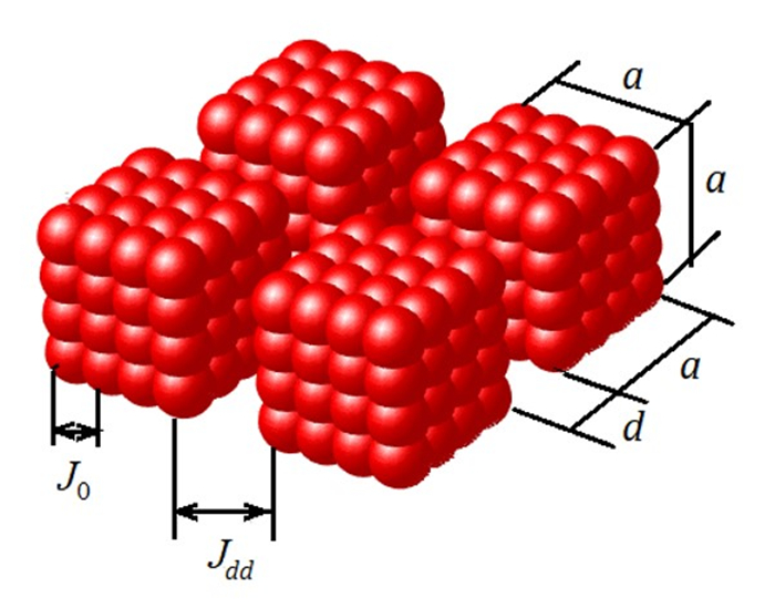
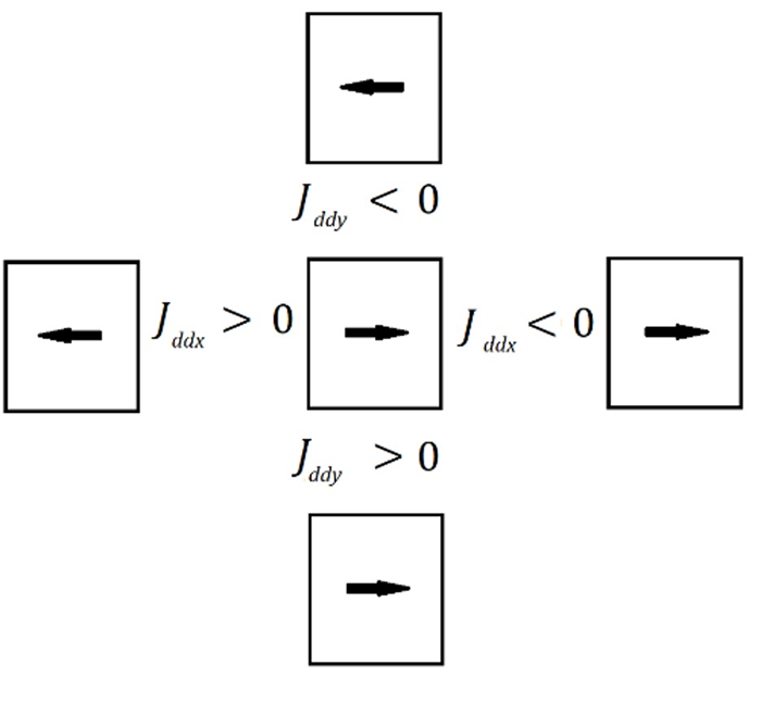
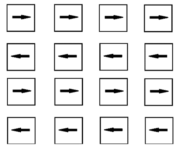
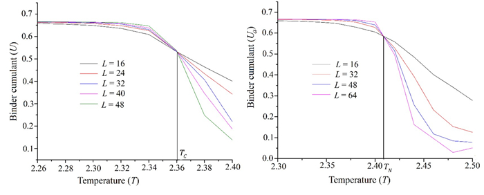
This article describes ordering in a 2D ferromagnetic nanoparticles array by computer simulation. The Heisenberg model simulates the behavior of spins in nanoparticles. Nanoparticles interact using dipole-dipole forces. Computer simulations use the Monte Carlo method and Metropolis algorithm. Two possible types of ordering for the nanoparticles' magnetic moments are detected in the system. The magnetic anisotropy direction for the nanoparticles determines the type of ordering. If the anisotropy direction is oriented perpendicular to the substrate plane, then a superantiferromagnetic phase with staggered magnetization is realized. If the magnetic anisotropy is oriented in the nanoparticle plane, the superantiferromagnetic phase has a different structure. The nanoparticle array is broken into chains parallel to the anisotropy orientations. In one chain of nanoparticles, magnetic moments are oriented in the same way. The magnetic moments of the nanoparticles are oriented oppositely in neighbor chains. The temperature of phase transitions is calculated based on finite dimensional scaling theory. Temperature depends linearly on the intensity of the dipole-dipole interaction for both types of superantiferromagnetic transition.
- ferromagnetic nanoparticles array,
- antiferromagnetic,
- phase transition,
- dipole-dipole interaction,
- computer simulation
Citation: Sergey V. Belim. Study of ordering in 2D ferromagnetic nanoparticles arrays: Computer simulation[J]. AIMS Materials Science, 2023, 10(6): 948-964. doi: 10.3934/matersci.2023051

Related Papers:

Abstract

This article describes ordering in a 2D ferromagnetic nanoparticles array by computer simulation. The Heisenberg model simulates the behavior of spins in nanoparticles. Nanoparticles interact using dipole-dipole forces. Computer simulations use the Monte Carlo method and Metropolis algorithm. Two possible types of ordering for the nanoparticles' magnetic moments are detected in the system. The magnetic anisotropy direction for the nanoparticles determines the type of ordering. If the anisotropy direction is oriented perpendicular to the substrate plane, then a superantiferromagnetic phase with staggered magnetization is realized. If the magnetic anisotropy is oriented in the nanoparticle plane, the superantiferromagnetic phase has a different structure. The nanoparticle array is broken into chains parallel to the anisotropy orientations. In one chain of nanoparticles, magnetic moments are oriented in the same way. The magnetic moments of the nanoparticles are oriented oppositely in neighbor chains. The temperature of phase transitions is calculated based on finite dimensional scaling theory. Temperature depends linearly on the intensity of the dipole-dipole interaction for both types of superantiferromagnetic transition.

References

[1]	Ehrmann A, Blachowicz T (2018) Systematic study of magnetization reversal in square Fe nanodots of varying dimensions in different orientations. Hyperfine Interact 239: 48. https://doi.org/10.1007/s10751-018-1523-1 doi: 10.1007/s10751-018-1523-1
[2]	Claridge SA, Castleman Jr AW, Khanna SN, et al. (2009) Cluster-assembled materials. ACS Nano 3: 244–255. https://oi.org/10.1021/nn800820e doi: 10.1021/nn800820e
[3]	Guo Y, Du Q, Wang P, et al. (2021) Two-dimensional oxides assembled by M₄ clusters (M = B, Al, Ga, In, Cr, Mo, and Te). Phys Rev Res 3: 043231. https://doi.org/10.1103/PhysRevResearch.3.043231 doi: 10.1103/PhysRevResearch.3.043231
[4]	Bista D, Sengupta T, Reber AC, et al. (2021) Interfacial magnetism in a fused superatomic cluster[Co₆Se₈(PEt₃)₅]₂. Nanoscale 13: 15763. https://doi.org/10.1039/d1nr00876e doi: 10.1039/d1nr00876e
[5]	Bramwell ST, Gingras MJ (2001) Spin ice state in frustrated magnetic pyrochlore materials. Science 294: 1495–1501. https://doi.org/10.1126/science.1064761 doi: 10.1126/science.1064761
[6]	Castelnovo C, Moessner R, Sondhi SL (2008) Magnetic monopoles in spin ice. Nature 451: 42–45. https://doi.org/10.1038/nature06433 doi: 10.1038/nature06433
[7]	Yumnam G, Guo J, Chen Y, et al. (2022) Magnetic charge and geometry confluence for ultra-low forward voltage diode in artificial honeycomb lattice. Mater Today Phys 22: 100574. https://doi.org/10.1016/j.mtphys.2021.100574 doi: 10.1016/j.mtphys.2021.100574
[8]	Keswani N, Singh R, Nakajima Y, et al. (2020) Accessing low-energy magnetic microstates in square artificial spin ice vertices of broken symmetry in static magnetic field. Phys Rev B 102: 224436. https://doi.org/10.1103/PhysRevB.102.224436 doi: 10.1103/PhysRevB.102.224436
[9]	Belim SV, Lyakh OV (2022) Phase transitions in an ordered 2D array of cubic nanoparticles. Lett Mater 12: 126–130. https://doi.org/10.22226/2410-3535-2022-2-126-130 doi: 10.22226/2410-3535-2022-2-126-130
[10]	Valdés DP, Lima E, Zysler R, et al. (2021) Role of anisotropy, frequency, and interactions in magnetic hyperthermia applications: Noninteracting nanoparticles and linear chain arrangements. Phys Rev Appl 15: 044005. https://doi.org/10.1103/PhysRevApplied.15.044005 doi: 10.1103/PhysRevApplied.15.044005
[11]	Li Y, Paterson GW, Macauley GM, et al. (2019) Superferromagnetism and domain-wall topologies in artificial "Pinwheel" spin ice. ACS Nano 13: 2213–2222. https://doi.org/10.1021/acsnano.8b08884 doi: 10.1021/acsnano.8b08884
[12]	Fuentes-García JA, Diaz-Cano AI, Guillen-Cervantes A, et al. (2018) Magnetic domain interactions of Fe₃O₄ nanoparticles embedded in a SiO₂ matrix. Sci Rep 8: 5096. https://doi.org/10.1038/s41598-018-23460-w doi: 10.1038/s41598-018-23460-w
[13]	Costanzo S, Ngo A, Russier V, et al. (2020) Enhanced structural and magneticproperties of fcc colloidal crystals of cobalt nanoparticles. Nanoscale 12: 24020–24029. https://doi.org/10.1039/D0NR05517D doi: 10.1039/D0NR05517D
[14]	Fedotova JA, Pashkevich AV, Ronassi AA, et al. (2020) Negative capacitance of nanocomposites with CoFeZr nanoparticles embedded into silica matrix. J Magn Magn Mat 511: 166963. https://doi.org/10.1016/j.jmmm.2020.166963 doi: 10.1016/j.jmmm.2020.166963
[15]	Kołtunowicz TN, Bondariev V, Zukowski P, et al. (2020) Ferromagnetic resonance spectroscopy of CoFeZr-CaF₂ granular nanocomposites. Prog Electromagn Res M 91: 11–18. https://doi.org/10.2528/PIERM19112107 doi: 10.2528/PIERM19112107
[16]	Timopheev AA, Ryabchenko SM, Kalita VM, et al. (2009) The influence of intergranular interaction on the magnetization of the ensemble of oriented Stoner-Wohlfarth nanoparticles. J Appl Phys 105: 083905. https://doi.org/10.1063/1.3098227 doi: 10.1063/1.3098227
[17]	Belim SV, Lyakh OV (2022) A study of a phase transition in an array of ferromagnetic nanoparticles with the dipole-dipole interaction using computer simulation. Phys Metals Metallogr 123: 1049–1053. https://doi.org/10.1134/S0031918X22601202 doi: 10.1134/S0031918X22601202
[18]	Nguyen MD, Tran HV, Xu S (2021) Fe₃O₄ nanoparticles: Structures, synthesis, magnetic properties, surface functionalization, and emerging applications. Appl Sci 11: 11301. https://doi.org/10.3390/app112311301 doi: 10.3390/app112311301
[19]	Köhler T, Feoktystov A, Petracic O, et al. (2021) Mechanism of magnetization reduction in iron oxide nanoparticles. Nanoscale 13: 6965–6976. https://doi.org/10.1039/D0NR08615K doi: 10.1039/D0NR08615K
[20]	Lemine OM, Madkhali N, Alshammari M, et al. (2021) Maghemite (γ-Fe₂O₃) and γ-Fe₂O₃-TiO₂ nanoparticles for magnetic hyperthermia applications: Synthesis, characterization and heating efficiency. Materials 14: 5691. https://doi.org/10.3390/ma14195691 doi: 10.3390/ma14195691
[21]	Batlle X, Moya C, Escoda-Torroella M, et al. (2022) Magnetic nanoparticles: From the nanostructure to the physical properties. J Magn Magn Mat 543: 168594. https://doi.org/10.1016/j.jmmm.2021.168594 doi: 10.1016/j.jmmm.2021.168594
[22]	Lazzarini A, Colaiezzi R, Passacantando M, et al. (2021) Investigation of physico-chemical and catalytic properties of the coating layer of silica-coated iron oxide magnetic nanoparticles. J Phys Chem Solids 153: 110003. https://doi.org/10.1016/j.jpcs.2021.110003 doi: 10.1016/j.jpcs.2021.110003
[23]	Ovejero JG, Spizzo F, Morales MP, et al. (2021) Mixing iron oxide nanoparticles with different shape and size for tunable magneto-heating performance. Nanoscale 13: 5714–5729. https://doi.org/10.1039/D0NR09121A doi: 10.1039/D0NR09121A
[24]	Li Y, Baberschke K (1992) Dimensional crossover in ultrathin Ni(111) films on W(110). Phys Rev Lett 68: 1208. https://doi.org/10.1103/PhysRevLett.68.1208 doi: 10.1103/PhysRevLett.68.1208
[25]	Prudnikov PV, Prudnikov VV, Medvedeva MA (2014) Dimensional effects in ultrathin magnetic films. Jetp Lett 100: 446–450. https://doi.org/10.1134/S0021364014190096 doi: 10.1134/S0021364014190096
[26]	Luis F, Bartolomé F, Petroff F, et al. (2006) Tuning the magnetic anisotropy of Co nanoparticles by metal capping. Europhys Lett 76: 142. https://doi.org/10.1209/epl/i2006-10242-2 doi: 10.1209/epl/i2006-10242-2
[27]	Landau DP, Binder K (1978) Phase diagrams and multicritical behavior of a three-dimensional anisotropic heisenberg antiferromagnet. Phys Rev B 17: 2328. https://doi.org/10.1103/PhysRevB.17.2328 doi: 10.1103/PhysRevB.17.2328
[28]	Binder K (1981) Critical properties from Monte-Carlo coarse-graining and renormalization. Phys Rev Lett 47: 693. https://doi.org/10.1103/PhysRevLett.47.693 doi: 10.1103/PhysRevLett.47.693
[29]	Lisjak D, Mertelj A (2018) Anisotropic magnetic nanoparticles: A review of their properties, syntheses and potential applications. Prog Mater Sci 95: 286–328. https://doi.org/10.1016/j.pmatsci.2018.03.003 doi: 10.1016/j.pmatsci.2018.03.003
[30]	Aquino VRR, Figueiredo LC, Coaquira JAH, et al. (2020) Magnetic interaction and anisotropy axes arrangement in nanoparticle aggregates can enhance or reduce the effective magnetic anisotropy. J Magn Magn Mat 498: 166170. https://doi.org/10.1016/j.jmmm.2019.166170 doi: 10.1016/j.jmmm.2019.166170
[31]	Gallina D, Pastor GM (2021) Structural disorder and collective behavior of two-dimensional magnetic nanostructures. Nanomaterials 11: 1392. https://doi.org/10.3390/nano11061392 doi: 10.3390/nano11061392
[32]	Gu E, Hope S, Tselepi M, et al. (1999) Two-dimensional paramagnetic-ferromagnetic phase transition and magnetic anisotropy in Co(110) epitaxial nanoparticle arrays. Phys Rev B 60: 4092. https://doi.org/10.1103/PhysRevB.60.4092 doi: 10.1103/PhysRevB.60.4092
[33]	Benitez MJ, Mishra D, Szary P, et al. (2011) Structural and magnetic characterization of self-assembled iron oxide nanoparticle arrays. J Phys Condens Matter 23: 126003. https://doi.org/10.1088/0953-8984/23/12/126003 doi: 10.1088/0953-8984/23/12/126003
[34]	Spasova M, Wiedwald U, Ramchal R, et al. (2002) Magnetic properties of arrays of interacting Co nanocrystals. J Magn Magn Mat 240: 40–43. https://doi.org/10.1016/S0304-8853(01)00723-5 doi: 10.1016/S0304-8853(01)00723-5
[35]	Schäffer AF, Sukhova A, Berakdar J (2017) Size-dependent frequency bands in the ferromagnetic resonance of a Fe-nanocube. J Magn Magn Mat 438: 70–75. https://doi.org/10.1016/j.jmmm.2017.04.065 doi: 10.1016/j.jmmm.2017.04.065
[36]	Morgunov RB, Koplak OV, Allayarov RS, et al. (2020) Effect of the stray field of Fe/Fe₃O₄ nanoparticles on the surface of the CoFeB thin films. Appl Surf Sci 527: 146836. https://doi.org/10.1016/j.apsusc.2020.146836 doi: 10.1016/j.apsusc.2020.146836
[37]	Ren H, Xiang G (2021) Morphology-dependent room-temperature ferromagnetism in undoped ZnO nanostructures. Nanomaterials 11: 3199. https://doi.org/10.3390/nano11123199 doi: 10.3390/nano11123199
[38]	Gao Y, Hou QY, Liu Y (2019) Effect of Fe doping and point defects (V_O and V_Sn) on the magnetic properties of SnO₂. J Supercond Nov Magn 32: 2877–2884. https://doi.org/10.1007/s10948-019-5053-0 doi: 10.1007/s10948-019-5053-0
[39]	Zhang C, Zhou M, Zhang Y, et al. (2019) Effects of oxygen vacancy on the magnetic properties of Ni-doped SnO₂ nanoparticles. J Supercond Nov Magn 32: 3509–3516. https://doi.org/10.1007/s10948-019-5094-4 doi: 10.1007/s10948-019-5094-4
[40]	Ming D, Xu L, Liu D, et al. (2008) Fabrication and phase transition of long-range-ordered, high-density GST nanoparticle arrays. Nanotechnology 19: 505304. https://doi.org/10.1088/0957-4484/19/50/505304 doi: 10.1088/0957-4484/19/50/505304
[41]	Vaz CAF, Bland JAC, Lauhoff G (2008) Magnetism in ultrathin film structures. Rep Prog Phys 71: 056501. https://doi.org/10.1088/0034-4885/71/5/056501 doi: 10.1088/0034-4885/71/5/056501

Reader Comments

Your name:*

Email:*
© 2023 the Author(s), licensee AIMS Press. This is an open access article distributed under the terms of the Creative Commons Attribution License (http://creativecommons.org/licenses/by/4.0)