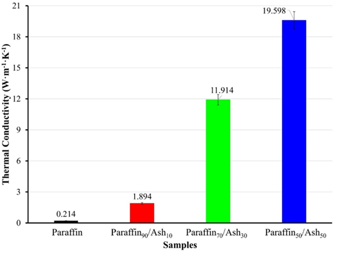
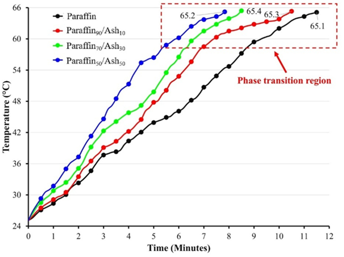
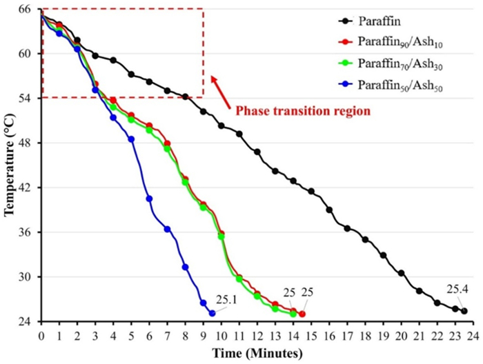
Low-temperature latent heat storage (LHS) systems are suitable for incorporating paraffin as the storage material. However, they face difficulty in actual implementation due to low thermal conductivity (TC). The present study used volcanic ash as an environmentally friendly and cost-effective material to increase the TC of paraffin. Three composites of paraffin/ash were prepared with ash proportions of 10 wt%, 30 wt% and 50 wt%. Characterizations were done to evaluate the average TC and properties. Thermal performance evaluation was conducted by analyzing the static charge/discharge cycle. The average TC for paraffin was 0.214 W/m·K. Adding volcanic ash improved the TC to 19.598 W/m·K. It made the charge/discharge performance of the composite better than that of pure paraffin. The charge rate for the composite ranged from 3.83 ℃/min to 5.12 ℃/min. The highest discharge rate was obtained at 4.21 ℃/min for the composite paraffin50/ash50. The freezing temperature for the composite is influenced by the ash proportion, which can be taken as a suitable approach to adjust the freezing point of paraffin-based thermal energy storage (TES). The detailed results for the characterization and thermal performance evaluation are described thoroughly within the article. The overall result indicates that volcanic ash is applicable for improving the TC and charge/discharge rate of paraffin-based TES.
Citation: Budhi Muliawan Suyitno, Dwi Rahmalina, Reza Abdu Rahman. Increasing the charge/discharge rate for phase-change materials by forming hybrid composite paraffin/ash for an effective thermal energy storage system[J]. AIMS Materials Science, 2023, 10(1): 70-85. doi: 10.3934/matersci.2023005
Low-temperature latent heat storage (LHS) systems are suitable for incorporating paraffin as the storage material. However, they face difficulty in actual implementation due to low thermal conductivity (TC). The present study used volcanic ash as an environmentally friendly and cost-effective material to increase the TC of paraffin. Three composites of paraffin/ash were prepared with ash proportions of 10 wt%, 30 wt% and 50 wt%. Characterizations were done to evaluate the average TC and properties. Thermal performance evaluation was conducted by analyzing the static charge/discharge cycle. The average TC for paraffin was 0.214 W/m·K. Adding volcanic ash improved the TC to 19.598 W/m·K. It made the charge/discharge performance of the composite better than that of pure paraffin. The charge rate for the composite ranged from 3.83 ℃/min to 5.12 ℃/min. The highest discharge rate was obtained at 4.21 ℃/min for the composite paraffin50/ash50. The freezing temperature for the composite is influenced by the ash proportion, which can be taken as a suitable approach to adjust the freezing point of paraffin-based thermal energy storage (TES). The detailed results for the characterization and thermal performance evaluation are described thoroughly within the article. The overall result indicates that volcanic ash is applicable for improving the TC and charge/discharge rate of paraffin-based TES.

| [1] |
Ismail I, Mulyanto AT, Rahman RA (2022) Development of free water knock-out tank by using internal heat exchanger for heavy crude oil. EUREKA: Phys Eng 77–85. https://doi.org/10.21303/2461-4262.2022.002502 doi: 10.21303/2461-4262.2022.002502

|
| [2] | Ismail I, Rahman RA, Haryanto G, et al. (2021) The optimal pitch distance for maximizing the power ratio for savonius turbine on inline configuration. IJRER 11: 595–599. |
| [3] | International Renewable Energy Agency (IRENA), Innovation outlook: Thermal energy storage, 2020. Available from: https://www.irena.org/Publications/2020/Nov/Innovation-outlook-Thermal-energy-storage. |
| [4] |
Ataei A (2016) Performance optimization of a combined solar collector, geothermal heat pump and thermal seasonal storage system for heating and cooling greenhouses. J Appl Eng Sci 14: 296–305. https://doi.org/10.5937/jaes14-8749 doi: 10.5937/jaes14-8749
|
| [5] |
Sadeghi G (2022) Energy storage on demand: Thermal energy storage development, materials, design, and integration challenges. Energy Storage Mater 46: 192-222. https://doi.org/10.1016/j.ensm.2022.01.017 doi: 10.1016/j.ensm.2022.01.017
|
| [6] |
Elbahjaoui R, El Qarnia H (2019) Performance evaluation of a solar thermal energy storage system using nanoparticle-enhanced phase change material. Int J Hydrogen Energ 44: 2013-2028. https://doi.org/10.1016/j.ijhydene.2018.11.116 doi: 10.1016/j.ijhydene.2018.11.116
|
| [7] |
Palacios A, Navarro ME, Barreneche C, et al. (2020) Hybrid 3 in 1 thermal energy storage system-Outlook for a novel storage strategy. Appl Energ 274: 115024. https://doi.org/10.1016/j.apenergy.2020.115024 doi: 10.1016/j.apenergy.2020.115024
|
| [8] |
Dsilva Winfred Rufuss D, Rajkumar V, Suganthi L, et al. (2019) Studies on latent heat energy storage (LHES) materials for solar desalination application-focus on material properties, prioritization, selection and future research potential. Sol Energ Mat Sol C 189: 149–165. https://doi.org/10.1016/j.solmat.2018.09.031 doi: 10.1016/j.solmat.2018.09.031
|
| [9] |
Yadav C, Sahoo RR (2019) Exergy and energy comparison of organic phase change materials based thermal energy storage system integrated with engine exhaust. J Energy Storage 24: 100773. https://doi.org/10.1016/j.est.2019.100773 doi: 10.1016/j.est.2019.100773
|
| [10] |
Rahmalina D, Rahman RA, Ismail I (2022) Improving the phase transition characteristic and latent heat storage efficiency by forming polymer-based shape-stabilized PCM for active latent storage system. Case Stud Therm Eng 101840. https://doi.org/10.1016/j.csite.2022.101840 doi: 10.1016/j.csite.2022.101840
|
| [11] |
Gandhi M, Kumar A, Elangovan R, et al. (2020) A review on shape-stabilized phase change materials for latent energy storage in buildings. Sustainability (Switzerland) 12: 1–17. https://doi.org/10.3390/su12229481 doi: 10.3390/su12229481
|
| [12] |
Wu S, Yan T, Kuai Z, et al. (2020) Thermal conductivity enhancement on phase change materials for thermal energy storage: A review. Energy Storage Mater 25: 251–295. https://doi.org/10.1016/j.ensm.2019.10.010 doi: 10.1016/j.ensm.2019.10.010
|
| [13] |
Rahmalina D, Rahman RA, Ismail (2022) Increasing the rating performance of paraffin up to 5000 cycles for active latent heat storage by adding high-density polyethylene to form shape-stabilized phase change material. J Energy Storage 46: 103762. https://doi.org/10.1016/j.est.2021.103762 doi: 10.1016/j.est.2021.103762
|
| [14] |
Ma X, Sheikholeslami M, Jafaryar M, et al. (2020) Solidification inside a clean energy storage unit utilizing phase change material with copper oxide nanoparticles. J Cleaner Production 245: 118888. https://doi.org/10.1016/j.jclepro.2019.118888 doi: 10.1016/j.jclepro.2019.118888
|
| [15] |
Zhang YP, Lin KP, Yang R, et al. (2006) Preparation, thermal performance and application of shape-stabilized PCM in energy efficient buildings. Energ Buildings 38: 1262–1269. https://doi.org/10.1016/j.enbuild.2006.02.009 doi: 10.1016/j.enbuild.2006.02.009
|
| [16] |
Yang X, Lu Z, Bai Q, et al. (2017) Thermal performance of a shell-and-tube latent heat thermal energy storage unit: Role of annular fins. Appl Energ 202: 558–570. https://doi.org/10.1016/j.apenergy.2017.05.007 doi: 10.1016/j.apenergy.2017.05.007
|
| [17] |
Waser R, Maranda S, Stamatiou A, et al. (2020) Modeling of solidification including supercooling effects in a fin-tube heat exchanger based latent heat storage. Sol Energy 200: 10–21. https://doi.org/10.1016/j.solener.2018.12.020 doi: 10.1016/j.solener.2018.12.020
|
| [18] |
Bayomy A, Davies S, Saghir Z (2019) Domestic hot water storage tank utilizing phase change materials (PCMs): Numerical approach. Energies 12: 2170. https://doi.org/10.3390/en12112170 doi: 10.3390/en12112170
|
| [19] |
Kalapala L, Devanuri JK (2018) Influence of operational and design parameters on the performance of a PCM based heat exchanger for thermal energy storage—A review. J Energ Storage 20: 497–519. https://doi.org/10.1016/j.est.2018.10.024 doi: 10.1016/j.est.2018.10.024
|
| [20] |
Deng Z, Li J, Zhang X, et al. (2020) Melting intensification in a horizontal latent heat storage (LHS) system using a paraffin/fractal metal matrices composite. J Energ Storage 32: 101857. https://doi.org/10.1016/j.est.2020.101857 doi: 10.1016/j.est.2020.101857
|
| [21] |
Chen P, Gao X, Wang Y, et al. (2016) Metal foam embedded in SEBS/paraffin/HDPE form-stable PCMs for thermal energy storage. Sol Energ Mater Sol C 149: 60–65. https://doi.org/10.1016/j.solmat.2015.12.041 doi: 10.1016/j.solmat.2015.12.041
|
| [22] |
Qu Y, Wang S, Zhou D, et al. (2020) Experimental study on thermal conductivity of paraffin-based shape-stabilized phase change material with hybrid carbon nano-additives. Renew Energ 146: 2637–2645. https://doi.org/10.1016/j.renene.2019.08.098 doi: 10.1016/j.renene.2019.08.098
|
| [23] |
Sheikholeslami M, Haq R ul, Shafee A, et al. (2019) Heat transfer simulation of heat storage unit with nanoparticles and fins through a heat exchanger. Int J Heat Mass Tran 135: 470–478. https://doi.org/10.1016/j.ijheatmasstransfer.2019.02.003 doi: 10.1016/j.ijheatmasstransfer.2019.02.003
|
| [24] |
Sciacovelli A, Navarro ME, Jin Y, et al. (2018) High density polyethylene (HDPE)-Graphite composite manufactured by extrusion: A novel way to fabricate phase change materials for thermal energy storage. Particuology 40: 131–140. https://doi.org/10.1016/j.partic.2017.11.011 doi: 10.1016/j.partic.2017.11.011
|
| [25] |
Játiva A, Ruales E, Etxeberria M (2021) Volcanic ash as a sustainable binder material: An extensive review. Materials 14: 1–32. https://doi.org/10.3390/ma14051302 doi: 10.3390/ma14051302
|
| [26] |
Kuznetsova E (2017) Thermal conductivity and the unfrozen water contents of volcanic ash deposits in cold climate conditions: A review. Clays Clay Miner 65: 168–183. https://doi.org/10.1346/CCMN.2017.064057 doi: 10.1346/CCMN.2017.064057
|
| [27] |
Rahmalina D, Adhitya DC, Rahman RA, et al. (2022) Improvement the performance of composite Pcm paraffin-based incorporate with volcanic ash as heat storage for low-temperature. EUREKA-Phys Eng 3–11. https://doi.org/10.21303/2461-4262.2022.002055 doi: 10.21303/2461-4262.2022.002055
|
| [28] | International Energy Agency Technology Collaboration Programme, Applications of thermal energy storage in the energy transition, 2018. Available from: https://iea-es.org/wp-content/uploads/public/86.3.3-IEA-ECES-Annex-30-Final-Report.pdf. |
| [29] |
Yinping Z, Yi J (1999) A simple method, the T-history method, of determining the heat of fusion, specific heat and thermal conductivity of phase-change materials. Meas Sci Technol 201–205. https://doi.org/10.1088/0957-0233/10/3/015 doi: 10.1088/0957-0233/10/3/015
|
| [30] |
Trisnadewi T, Kusrini E, Nurjaya DM, et al. (2021) Experimental analysis of natural wax as phase change material by thermal cycling test using thermoelectric system. J Energy Storage 40: 102703. https://doi.org/10.1016/j.est.2021.102703 doi: 10.1016/j.est.2021.102703
|
| [31] |
Eanest Jebasingh B, Valan Arasu A (2020) A comprehensive review on latent heat and thermal conductivity of nanoparticle dispersed phase change material for low-temperature applications. Energy Storage Mater 24: 52–74. https://doi.org/10.1016/j.ensm.2019.07.031 doi: 10.1016/j.ensm.2019.07.031
|
| [32] |
Shamseddine I, Pennec F, Biwole P, et al. (2022) Supercooling of phase change materials: A review. Renewa Sust Energ Rev 158: 112172. https://doi.org/10.1016/j.rser.2022.112172 doi: 10.1016/j.rser.2022.112172
|
| [33] |
Tabassum T, Hasan M, Begum L (2018) Transient melting of an impure paraffin wax in a double-pipe heat exchanger: Effect of forced convective flow of the heat transfer fluid. Sol Energy 159: 197–211. https://doi.org/10.1016/j.solener.2017.10.082 doi: 10.1016/j.solener.2017.10.082
|
| [34] |
Liu L, Zhang X, Xu X, et al. (2020) The research progress on phase change hysteresis affecting the thermal characteristics of PCMs: A review. J Mol Liq 317: 113760. https://doi.org/10.1016/j.molliq.2020.113760 doi: 10.1016/j.molliq.2020.113760
|
| [35] |
Rahman RA, Lahuri AH, Ismail I (2023) Thermal stress influence on the long-term performance of fast-charging paraffin-based thermal storage. TSEP 37: 101546. https://doi.org/10.1016/j.tsep.2022.101546 doi: 10.1016/j.tsep.2022.101546
|
Figures(8)

Budhi Muliawan Suyitno, Dwi Rahmalina, Reza Abdu Rahman. Increasing the charge/discharge rate for phase-change materials by forming hybrid composite paraffin/ash for an effective thermal energy storage system[J]. AIMS Materials Science, 2023, 10(1): 70-85. doi: 10.3934/matersci.2023005


 DownLoad: