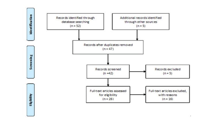
Polydimethylsiloxane mechanical properties: A systematic review

Inês Teixeira; Inês Castro; Violeta Carvalho; Cristina Rodrigues; Andrews Souza; Rui Lima; Senhorinha Teixeira; João Ribeiro; Inês Teixeira; Inês Castro; Violeta Carvalho; Cristina Rodrigues; Andrews Souza; Rui Lima; Senhorinha Teixeira; João Ribeiro

doi:10.3934/matersci.2021058

AIMS Materials Science

2021, Volume 8, Issue 6: 952-973. doi: 10.3934/matersci.2021058

Previous Article Next Article

Review Topical Sections

Polydimethylsiloxane mechanical properties: A systematic review

1.
University of Minho, Mechanical Engineering Department, University of Minho, Campus de Azurém, Guimarães, Portugal
2.
MEtRICs, Mechanical Engineering Department, University of Minho, Campus de Azurém, Guimarães, Portugal
3.
ALGORITMI, Production and Systems Department, School of Engineering, University of Minho, Campus de Azurém, Guimarães, Portugal
4.
Instituto Politécnico de Bragança, Campus Sta Apolónia, Bragança, Portugal
5.
CIMO, Campus Sta Apolónia, 5300-253 Bragança, Portugal

Received: 08 July 2021 Accepted: 29 November 2021 Published: 20 December 2021

Polydimethylsiloxane (PDMS) has been a promising material for microfluidic, particularly in lab-on-chip. Due to the panoply of good physical, mechanical and chemical properties, namely, viscosity, modulus of elasticity, colour, thermal conductivity, thermal coefficient of expansion, its application has been increasingly requested in quite different areas. Despite such characteristics, there are also some drawbacks associated, and to overcome them, several strategies have been developed to modify PDMS. Given the great variety of relevant conducted research in this field, the present work aims to gather the most relevant information, the advantages and disadvantages of some of the techniques used, and also identify potential gaps and challenges in it. To this end, a systematic literature review was conducted by collecting data from four different databases, Science Direct, American Chemical Society, Scopus, and Springer. Two authors independently screened the references, extracted the key information, and assessed the quality of the included studies. After the analysis of the collected data, 25 studies were selected that addressed the various mechanical properties of PDMS and how to modify them in order to suit a particular application.
- materials modification,
- mechanical properties,
- organic polymer,
- PDMS properties,
- polydimethylsiloxane
Citation: Inês Teixeira, Inês Castro, Violeta Carvalho, Cristina Rodrigues, Andrews Souza, Rui Lima, Senhorinha Teixeira, João Ribeiro. Polydimethylsiloxane mechanical properties: A systematic review[J]. AIMS Materials Science, 2021, 8(6): 952-973. doi: 10.3934/matersci.2021058

Related Papers:

Abstract

Polydimethylsiloxane (PDMS) has been a promising material for microfluidic, particularly in lab-on-chip. Due to the panoply of good physical, mechanical and chemical properties, namely, viscosity, modulus of elasticity, colour, thermal conductivity, thermal coefficient of expansion, its application has been increasingly requested in quite different areas. Despite such characteristics, there are also some drawbacks associated, and to overcome them, several strategies have been developed to modify PDMS. Given the great variety of relevant conducted research in this field, the present work aims to gather the most relevant information, the advantages and disadvantages of some of the techniques used, and also identify potential gaps and challenges in it. To this end, a systematic literature review was conducted by collecting data from four different databases, Science Direct, American Chemical Society, Scopus, and Springer. Two authors independently screened the references, extracted the key information, and assessed the quality of the included studies. After the analysis of the collected data, 25 studies were selected that addressed the various mechanical properties of PDMS and how to modify them in order to suit a particular application.

References

[1]	Wu CL, Lin HC, Hsu JS, et al. (2009) Static and dynamic mechanical properties of polydimethylsiloxane/carbon nanotube nanocomposites. Thin Solid Films 517: 4895-4901.
[2]	Xu W, Chahine N, Sulchek T (2011) Extreme hardening of PDMS thin films due to high compressive strain and confined thickness. Langmuir 27: 8470-8477.
[3]	Klasner SA, Metto EC, Roman GT, et al. (2009) Synthesis and characterization of a poly(dimethylsiloxane)-poly(ethylene oxide) block copolymer for fabrication of amphiphilic surfaces on microfluidic devices. Langmuir 25: 10390-10396.
[4]	Zahid A, Dai B, Hong R, et al. (2017) Optical properties study of silicone polymer PDMS substrate surfaces modified by plasma treatment. Mater Res Express 4: 105301.
[5]	Vlassov S, Oras S, Antsov M, et al. (2018) Adhesion and mechanical properties of PDMS-based materials probed with AFM: A review. Rev Adv Mater Sci 56: 62-78.
[6]	Carvalho V, Gonçalves I, Lage T, et al. (2021) 3D printing techniques and their applications to organ‐on‐a‐chip platforms: A systematic review. Sensors 21: 3304.
[7]	Carvalho V, Maia I, Souza A, et al. (2021) In vitro biomodels in stenotic arteries to perform blood analogues flow visualizations and measurements: A review. Open Biomed Eng J 14: 87-102.
[8]	Kacik D, Martincek I (2017) Toluene optical fibre sensor based on air microcavity in PDMS. Opt Fiber Technol 34: 70-73.
[9]	Park JS, Cabosky R, Ye Z, et al. (2018) Investigating the mechanical and optical properties of thin PDMS film by flat-punched indentation. Opt Mater 85: 153-161.
[10]	A Souza, E Marques, C Balsa, et al. (2020) Characterization of shear strain on PDMS: Numerical and experimental approaches. Appl Sci 10: 3322.
[11]	Montazerian H, Mohamed MGA, Montazeri MM, et al. (2019) Permeability and mechanical properties of gradient porous PDMS scaffolds fabricated by 3D-printed sacrificial templates designed with minimal surfaces. Acta Biomater 96: 149-160.
[12]	Lamberti A, Marasso SL, Cocuzza MJR (2014) PDMS membranes with tunable gas permeability for microfluidic applications. RSC Adv 4: 61415-61419.
[13]	Firpo G, Angeli E, Repetto L, et al. (2015) Permeability thickness dependence of polydimethylsiloxane (PDMS) membranes. J Membrane Sci 481: 1-8.
[14]	Keane TJ, Badylak SF (2014) Biomaterials for tissue engineering applications. Semin Pediatr Surg 23: 112-118.
[15]	Shi Y, Hu M, Xing Y, et al. (2020) Temperature-dependent thermal and mechanical properties of flexible functional PDMS/paraffin composites. Mater Des 185: 108219.
[16]	Pinho D, Muñ oz-Sánchez BN, Anes CF, et al. (2019) Flexible PDMS microparticles to mimic RBCs in blood particulate analogue fluids. Mech Res Commun 100: 103399.
[17]	Giri R, Naskar K, Nando GB (2012) Effect of electron beam irradiation on dynamic mechanical, thermal and morphological properties of LLDPE and PDMS rubber blends. Radiat Phys Chem 81: 1930-1942.
[18]	Dalla Monta A, Razan F, Le Cam JB, et al. (2018) Using thickness-shear mode quartz resonator for characterizing the viscoelastic properties of PDMS during cross-linking, from the liquid to the solid state and at different temperatures. Sensor Actuat-A Phys 280: 107-113.
[19]	Li J, Wang M, Shen Y (2012) Chemical modification on top of nanotopography to enhance surface properties of PDMS. Surf Coat Tech 206: 2161-2167.
[20]	Yang C, Yuan YJ (2016) Investigation on the mechanism of nitrogen plasma modified PDMS bonding with SU-8. Appl Surf Sci 364: 815-821.
[21]	Sales F, Souza A, Ariati R, et al. (2021) Composite material of PDMS with interchangeable transmittance: Study of optical, mechanical properties and wettability. J Compos Sci 5: 1-13.
[22]	Ressel J, Seewald O, Bremser W, et al. (2020) Self-lubricating coatings via PDMS micro-gel dispersions. Prog Org Coat 146: 105705.
[23]	Syafiq A, Vengadaesvaran B, Rahim NA, et al. (2019) Transparent self-cleaning coating of modified polydimethylsiloxane (PDMS) for real outdoor application. Prog Org Coat 131: 232-239.
[24]	Park JY, Song H, Kim T, et al. (2016) PDMS-paraffin/graphene laminated films with electrothermally switchable haze. Carbon 96: 805-811.
[25]	Wang W, Fang J (2007) Variable focusing microlens chip for potential sensing applications. IEEE Sens J 7: 11-17.
[26]	Sadek SH, Rubio M, Lima R, et al. (2021) Blood particulate analogue fluids: A review. Materials 14: 2451.
[27]	Wu X, Kim SH, Ji CH, et al. (2011) A solid hydraulically amplified piezoelectric microvalve. J Micromech Microeng 21: 095003.
[28]	Maram SK, Barron B, Leung JC, et al. (2018) Fabrication and thermoresistive behaviour characterization of three-dimensional silver-polydimethylsiloxane (Ag-PDMS) microbridges in a mini-channel. Sensor Actuat A-Phys 277: 43-51.
[29]	Akther F, Yakob SB, Nguyen NT, et al. (2020) Surface modification techniques for endothelial cell seeding in PDMS microfluidic devices. Biosensors 10: 182.
[30]	Catarino SO, Rodrigues RO, Pinho D, et al. (2019) Blood cells separation and sorting techniques of passive microfluidic devices: From fabrication to applications. Micromachines 10: 593.
[31]	Wolf MP, Salieb-Beugelaar GB, Hunziker P (2018) PDMS with designer functionalities—Properties, modifications strategies, and applications. Prog Polym Sci 83: 97-134.
[32]	Anisimov AA, Zaytsev AV, Ol'shevskaya VA, et al. (2016) Polydimethylsiloxanes with bulk end groups: Synthesis and properties. Mendeleev Commun 26: 524-526.
[33]	Ribeiro JE, Lopes H, Martins P, et al. (2019) Mechanical analysis of PDMS material using biaxial test. AIMS Mater Sci 6: 97-110.
[34]	Victor A, Ribeiro JE, Araújo FF (2019) Study of PDMS characterization and its applications in biomedicine: A review. J Mech Eng Biomech 4: 1-9.
[35]	Mata A, Fleischman AJ, Roy S (2005) Characterization of polydimethylsiloxane (PDMS) properties for biomedical micro/nanosystems. Biomed Microdevices 2: 281-293.
[36]	Johnston ID, McCluskey DK, Tan CKL, et al. (2014) Mechanical characterization of bulk Sylgard 184 for microfluidics and microengineering. J Micromech Microeng 24: 035017.
[37]	Kalulu M, Zhang W, Xia XK, et al. (2018) Hydrophilic surface modification of polydimetylsiloxane‐co‐2‐hydroxyethylmethacrylate (PDMS‐HEMA) by Silwet L‐77 (heptamethyltrisiloxane) surface treatment. Polym Adv Technol 29: 2601-2611.
[38]	Gökaltun A, Kang YBA, Yarmush ML, et al. (2019) Simple surface modification of poly(dimethylsiloxane) via surface segregating smart polymers for biomicrofluidics. Sci Rep 9: 1-14.
[39]	Bodas D, Rauch JY, Khan-Malek C (2008) Surface modification and aging studies of addition-curing silicone rubbers by oxygen plasma. Eur Polym J 44: 2130-2139.
[40]	Bhattacharya S, Datta A, Berg JM, et al. (2005) Studies on surface wettability of poly(dimethyl) siloxane (PDMS) and glass under oxygen-plasma treatment and correlation with bond strength. J Microelectromech S 14: 590-597.
[41]	Seethapathy S, Górecki T (2012) Applications of polydimethylsiloxane in analytical chemistry: A review. Anal Chim Acta 750: 48-62.
[42]	Souza A, Souza MS, Pinho D, et al. (2020) 3D manufacturing of intracranial aneurysm biomodels for flow visualizations: Low cost fabrication processes. Mech Res Commun 107: 103535.
[43]	Rodrigues RO, Pinho D, Bento D, et al. (2016) Wall expansion assessment of an intracranial aneurysm model by a 3D digital image correlation system. Measurement 88: 262-270.
[44]	Rodrigues RO, Sousa PC, Gaspar J, et al. (2020) Organ-on-a-chip: A preclinical microfluidic platform for the progress of nanomedicine. Small 16: 2003517.
[45]	Eduok U, Faye O, Szpunar J (2017) Recent developments and applications of protective silicone coatings: A review of PDMS functional materials. Prog Org Coat 111: 124-163.
[46]	Russell MT, Pingree LSC, Hersam MC, et al. (2006) Microscale features and surface chemical functionality patterned by electron beam lithography: A novel route to poly(dimethylsiloxane) (PDMS) stamp fabrication. Langmuir 22: 6712-6718.
[47]	Lötters JC, Olthuis W, Veltink PH, et al. (1997) The mechanical properties of the rubber elastic polymer polydimethylsiloxane for sensor applications. J Micromech Microeng 7: 145-147.
[48]	Mohamed NS, Theng KC (2019) Mechanical properties of graded polydimethylsiloxane for flexible electronics. J Phys Conf Ser 1150: 012030.
[49]	Lai HY, Wang HQ, Lai JC, et al. (2019) A self-healing and shape memory polymer that functions at body temperature. Molecules 24: 3224.
[50]	Xu CA, Lu M, Tan Z, et al. (2020) Study on the surface properties and thermal stability of polysiloxane-based polyurethane elastomers with aliphatic and aromatic diisocyanate structures. Colloid Polym Sci 298: 1215-1226.
[51]	Kim JH, Lee J, Kim W, et al. (2019) Characterization of viscoelastic behaviour of poly(dimethylsiloxane) by nanoindentation. Korean J Met Mater 57: 289-294.
[52]	Kherroub DE, Boulaouche T (2020) Maghnite: Novel inorganic reinforcement for single-step synthesis of PDMS nanocomposites with improved thermal, mechanical and textural properties. Res Chem Intermed 46: 5199-5217.
[53]	Queiroz DP, De Pinho MN (2005) Structural characteristics and gas permeation properties of polydimethylsiloxane/poly(propylene oxide) urethane/urea bi-soft segment membranes. Polymer 46: 2346-2353.
[54]	Lin X, Park S, Choi D, et al. (2019) Mechanically durable superhydrophobic PDMS-candle soot composite coatings with high biocompatibility. J Ind Eng Chem 74: 79-85.
[55]	Atthi N, Sripumkhai W, Pattamang P, et al. (2020) Superhydrophobic and superoleophobic properties enhancement on PDMS micro-structure using simple flame treatment method. Microelectron Eng 230: 111362.
[56]	Cai JH, Huang ML, Chen XD, et al. (2021) Thermo-expandable microspheres strengthened polydimethylsiloxane foam with unique softening behaviour and high-efficient energy absorption. Appl Surf Sci 540: 148364.
[57]	Berkem AS, Capoglu A, Nugay T, et al. (2018) Self-healable supramolecular vanadium pentoxide reinforced polydimethylsiloxane-graft-polyurethane composites. Polymers 11: 18-20.
[58]	Goyal A, Kumar A, Patra PK, et al. (2009) In situ synthesis of metal nanoparticle embedded free standing multifunctional PDMS films. Macromol Rapid Commun 30: 1116-1122.
[59]	Konku-Asase Y, Yaya A, Kan-Dapaah K (2020) Curing temperature effects on the tensile properties and hardness of γ-Fe₂O₃ reinforced PDMS nanocomposites. Adv Mater Sci Eng 2020.
[60]	Liu J, Zong G, He L, et al. (2015) Effects of fumed and mesoporous silica nanoparticles on the properties of sylgard 184 polydimethylsiloxane. Micromachines 6: 855-864.
[61]	Shafaamri A, Cheng CH, Wonnie Ma IA, et al. (2020) Effects of TiO₂ nanoparticles on the overall performance and corrosion protection ability of neat epoxy and PDMS modified epoxy coating systems. Front Mater 6: 336.
[62]	Fojtíková J, Kalvoda L (2018) Molecular dynamics simulations of poly(dimethylsiloxane) elasticity. Acta Phys Pol A 134: 857-858.
[63]	Mata A, Fleischman AJ, Roy S (2005) Characterization of polydimethylsiloxane (PDMS) properties for biomedical micro/nanosystems. Biomed Microdevices 7: 281-293.
[64]	Zhang G, Sun Y, Qian B, et al. (2020) Experimental study on mechanical performance of polydimethylsiloxane (PDMS) at various temperatures. Polym Test 90: 106670.
[65]	Liu M, Sun J, Chen Q (2009) Influences of heating temperature on mechanical properties of polydimethylsiloxane. Sensor Actuat A-Phys 151: 42-45.

Reader Comments

Your name:*

Email:*
© 2021 the Author(s), licensee AIMS Press. This is an open access article distributed under the terms of the Creative Commons Attribution License (http://creativecommons.org/licenses/by/4.0)