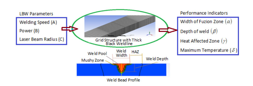
Day by day laser welding (LW) is gaining industrial importance. Good quality of weld joints can be realized through this process. Because this process yields low distortion and small weld bead. Aerospace, nuclear, automotive, and biomedical industries are opting for the lightweight and corrosion resistance titanium alloys. This paper deals with the generation of optimal weld bead profiles in the conduction mode laser beam welding (LBW) of thin Ti–6Al–4V alloy sheets. Laser beam diameter, power and welding speed are the 3 LBW parameters, whereas, bead width, depth of penetration, heat affected zone and maximum temperature are the performance indicators (PIs). 3 levels are set for each LBW parameter. Taguchi's L9 OA (orthogonal array) is selected to minimize the numerical simulations. ANSYS Fluent V16.0 with Vc++ code is used to develop a generic model. %Contribution of each process variable on the PIs is assessed performing ANOVA analysis. The range of PIs is assessed adopting the modified Taguchi approach. A set of optimal LBW parameters are identified considering a multi-objective optimization technique. For these optimal LBW parameters weld bead width is minimum, and the depth of penetration is maximum. Empirical relations for PIs are developed and validated with simulations. Utilizing the Taguchi's design of experiments, empirical relations are developed for the performance indicators in laser beam welding (LBW) simulations performing few trial runs and identified the optimal LBW process parameters.
Citation: Harish Mooli, Srinivasa Rao Seeram, Satyanarayana Goteti, Nageswara Rao Boggarapu. Optimal weld bead profiles in the conduction mode LBW of thin Ti–6Al–4V alloy sheets[J]. AIMS Materials Science, 2021, 8(5): 698-715. doi: 10.3934/matersci.2021042
Day by day laser welding (LW) is gaining industrial importance. Good quality of weld joints can be realized through this process. Because this process yields low distortion and small weld bead. Aerospace, nuclear, automotive, and biomedical industries are opting for the lightweight and corrosion resistance titanium alloys. This paper deals with the generation of optimal weld bead profiles in the conduction mode laser beam welding (LBW) of thin Ti–6Al–4V alloy sheets. Laser beam diameter, power and welding speed are the 3 LBW parameters, whereas, bead width, depth of penetration, heat affected zone and maximum temperature are the performance indicators (PIs). 3 levels are set for each LBW parameter. Taguchi's L9 OA (orthogonal array) is selected to minimize the numerical simulations. ANSYS Fluent V16.0 with Vc++ code is used to develop a generic model. %Contribution of each process variable on the PIs is assessed performing ANOVA analysis. The range of PIs is assessed adopting the modified Taguchi approach. A set of optimal LBW parameters are identified considering a multi-objective optimization technique. For these optimal LBW parameters weld bead width is minimum, and the depth of penetration is maximum. Empirical relations for PIs are developed and validated with simulations. Utilizing the Taguchi's design of experiments, empirical relations are developed for the performance indicators in laser beam welding (LBW) simulations performing few trial runs and identified the optimal LBW process parameters.

| [1] |
Oliveira JP, Schell N, Zhou N, et al. (2019) Laser welding of precipitation strengthened Ni-rich NiTiHf high temperature shape memory alloys: Microstructure and mechanical properties. Mater Design 162: 229-234. doi: 10.1016/j.matdes.2018.11.053

|
| [2] |
Oliveira JP, Shen J, Escobar JD, et al. (2021) Laser welding of H-phase strengthened Ni-rich NiTi-20Zr high temperature shape memory alloy. Mater Design 202: 109533. doi: 10.1016/j.matdes.2021.109533
|
| [3] |
Shamsolhodaei A, Oliveira JP, Schell N, et al. (2020) Controlling intermetallic compounds formation during laser welding of NiTi to 316L stainless steel. Intermetallics 116: 106656. doi: 10.1016/j.intermet.2019.106656
|
| [4] |
Wang SH, Wei MD, Tsay LW (2003) Tensile properties of LBW welds in Ti-6Al-4V alloy at evaluated temperatures below 450 º С. Mater Lett 57: 1815-1823. doi: 10.1016/S0167-577X(02)01074-1
|
| [5] |
Auwal ST, Ramesh S, Yusof F, et al. (2018) A review on laser beam welding of titanium alloys. Int J Adv Manuf Technol 97: 1071-1098. doi: 10.1007/s00170-018-2030-x
|
| [6] | Denney PE, Metzbower EA (1989) Laser beam welding of titanium. Weld J 68: 342-346. |
| [7] |
Du H, Hu L, Liu J, et al. (2004) A study on the metal flow in full penetration laser beam welding for titanium alloy. Comp Mater Sci 29: 419-427. doi: 10.1016/j.commatsci.2003.11.002
|
| [8] |
Benyounis KY, Olabi AG, Hashmi MSJ (2005) Effect of laser welding parameters on the heat input and weld-bead profile. J Mater Process Tech 164: 978-985. doi: 10.1016/j.jmatprotec.2005.02.060
|
| [9] |
Liao YC, Yu MH (2007) Effects of laser beam energy and incident angle on the pulse laser welding of stainless steel thin sheet. J Mater Process Tech 190: 102-108. doi: 10.1016/j.jmatprotec.2007.03.102
|
| [10] |
Akman E, Demir A, Canel T, et al. (2009) Laser welding of Ti6Al4V titanium alloys. J Mater Process Tech 209: 3705-3713. doi: 10.1016/j.jmatprotec.2008.08.026
|
| [11] |
Khorram A, Yazdi MRS, Ghoreishi M, et al. (2010) Using ANN approach to investigate the weld geometry of Ti 6Al 4V Titanium Alloy. Int J Eng Technol 2: 491. doi: 10.7763/IJET.2010.V2.170
|
| [12] | Yamashita S, Yonemoto Y, Yamada T, et al. (2010) Numerical simulation of laser welding processes with CIP finite volume method. Trans JWRI 39: 37-39. |
| [13] | Takemori CK, Muller DT, Oliveira MA (2010) Numerical simulation of transient heat transfer during welding process. International Compressor Engineering Conference at Purdue, 1-8. |
| [14] |
Sathiya P, Jaleel MYA, Katherasan D, et al. (2011) Optimization of laser butt welding parameters with multiple performance characteristics. Opt Laser Technol 43: 660-673. doi: 10.1016/j.optlastec.2010.09.007
|
| [15] |
Shanmugam NS, Buvanashekaran G, Sankaranarayanasamy K (2012) Some studies on weld bead geometries for laser spot welding process using finite element analysis. Mater Design 34: 412-426. doi: 10.1016/j.matdes.2011.08.005
|
| [16] |
Squillace A, Prisco U, Ciliberto S, et al. (2012) Effect of welding parameters on morphology and mechanical properties of Ti-6Al-4V laser beam welded butt joints. J Mater Process Tech 212: 427-436. doi: 10.1016/j.jmatprotec.2011.10.005
|
| [17] |
Cherepanov AN, Shapeev VP, Liu G, et al. (2012) Simulation of thermophysical processes at laser welding of alloys containing refractory nanoparticles. AMPC 2: 270-273. doi: 10.4236/ampc.2012.24B069
|
| [18] |
Cao X, Kabir ASH, Wanjara P, et al. (2014) Global and local mechanical properties of autogenously laser welded Ti-6Al-4V. Metall Mater Trans A 45: 1258-1272. doi: 10.1007/s11661-013-2106-z
|
| [19] | Song SP, Paradowska AM, Dong PS (2014) Investigation of residual stresses distribution in titanium weldments, Materials Science Forum, 777: 171-175. |
| [20] |
Akbari M, Saedodin S, Toghraie D, et al. (2014) Experimental and numerical investigation of temperature distribution and melt pool geometry during pulsed laser welding of Ti6Al4V alloy. Opt Laser Technol 59: 52-59. doi: 10.1016/j.optlastec.2013.12.009
|
| [21] |
Gao XL, Zhang LJ, Liu J, et al. (2014) Porosity and microstructure in pulsed Nd:YAG laser welded Ti6Al4V sheet. J Mater Process Tech 214: 1316-1325. doi: 10.1016/j.jmatprotec.2014.01.015
|
| [22] |
Gao XL, Liu J, Zhang LJ, et al. (2014) Effect of the overlapping factor on the microstructure and mechanical properties of pulsed Nd:YAG laser welded Ti6Al4V sheets. Mater Charact 93: 136-149. doi: 10.1016/j.matchar.2014.04.005
|
| [23] | Azizpour M, Ghoreishi M, Khorram A (2015) Numerical simulation of laser beam welding of Ti6Al4V sheet. JCARME 4: 145-154. |
| [24] | Akbari M, Saedodin S, Panjehpour A, et al. Numerical simulation and designing artificial neural network for estimating melt pool geometry and temperature distribution in laser welding of Ti6Al4V alloy. Optik 127: 11161-11172. |
| [25] |
Zhan X, Li Y, Ou W, et al. (2016) Comparison between hybrid laser-MIG welding and MIG welding for the invar36 alloy. Opt Laser Technol 85: 75-84. doi: 10.1016/j.optlastec.2016.06.001
|
| [26] |
Zhan X, Peng Q, Wei Y, et al. (2017) Experimental and simulation study on the microstructure of TA15 titanium alloy laser beam welded joints. Opt Laser Technol 94: 279-289. doi: 10.1016/j.optlastec.2017.03.014
|
| [27] |
Oliveira JP, Miranda RM, Fernandes FMB (2017) Welding and joining of NiTi shape memory alloys: a review. Prog Mater Sci 88: 412-466. doi: 10.1016/j.pmatsci.2017.04.008
|
| [28] |
Oliveira JP, Panton B, Zeng Z, et al. (2016) Laser joining of NiTi to Ti6Al4V using a Niobium interlayer. Acta Mater 105: 9-15. doi: 10.1016/j.actamat.2015.12.021
|
| [29] |
Su C, Zhou JZ, Ye YX, et al. (2017) Study on fiber laser welding of AA6061-T6 samples through numerical simulation and experiments. Procedia Eng 174: 732-739. doi: 10.1016/j.proeng.2017.01.213
|
| [30] |
Gursel A (2017) Crack risk in Nd: YAG laser welding of Ti-6Al-4V alloy. Mater Lett 197: 233-235. doi: 10.1016/j.matlet.2016.12.112
|
| [31] | Caiazzo F, Alfieri V, Astarita A, et al. (2016) Investigation on laser welding of Ti-6Al-4V plates in corner joint. Adv Mech Eng 9: 1-9. |
| [32] |
Kumar C, Das M, Paul CP, et al. (2017) Experimental investigation and metallographic characterization of fiber laser beam welding of Ti-6Al-4V alloy using response surface method. Opt Laser Eng 95: 52-68. doi: 10.1016/j.optlaseng.2017.03.013
|
| [33] |
Kumar U, Gope DK, Srivastava JP, et al. (2018) Experimental and numerical assessment of temperature field and analysis of microstructure and mechanical properties of low power laser annealed welded joints. Materials 11: 1514. doi: 10.3390/ma11091514
|
| [34] |
Auwal ST, Ramesh S, Yusof F, et al. (2018) A review on laser beam welding of titanium alloys. Int J Adv Manuf Technol 97: 1071-1098. doi: 10.1007/s00170-018-2030-x
|
| [35] |
Kumar GS, Raghukandan K, Saravanan S, et al. (2019) Optimization of parameters to attain higher tensile strength in pulsed Nd:YAG laser welded Hastelloy C-276-Monel 400 sheets. Infrared Phys Techn 100: 1-10. doi: 10.1016/j.infrared.2019.05.002
|
| [36] |
Jiang D, Alsagri AS, Akbari M, et al. (2019) Numerical and experimental studies on the effect of varied beam diameter, average power and pulse energy in Nd:YAG laser welding of Ti6Al4V. Infrared Phys Techn 101: 180-188. doi: 10.1016/j.infrared.2019.06.006
|
| [37] |
Kumar P, Sinha AN (2019) Effect of heat input in pulsed Nd:YAG laser welding of titanium alloy (Ti6Al4V) on microstructure and mechanical properties. Weld World 63: 673-689. doi: 10.1007/s40194-018-00694-w
|
| [38] | Steen WM, Mazumder J (2010) Laser Material Processing, 4 Eds., Berlin: Springer Science & Business Media. |
| [39] | Assuncao DE, Ganguly S, Yapp D, et al. (2010) Conduction mode: broadening the range of applications for laser welding. 63rd Annual Assembly & International Conference of the International Institute of Welding, Istanbul, Turkey, 705-709. |
| [40] | Shao J, Yan Y (2005) Review of techniques for on-line monitoring and inspection of laser welding, Journal of Physics: Conference Series, 15: 017. |
| [41] |
He X (2012) Finite element analysis of laser welding: a state of art review. Mater Manuf Process 27: 1354-1365. doi: 10.1080/10426914.2012.709345
|
| [42] |
Satyanarayana G, Narayana KL, Boggarapu NR (2018) Numerical simulations on the laser spot welding of zirconium alloy endplate for nuclear fuel bundle assembly. Lasers Manuf Mater Process 5: 53-70. doi: 10.1007/s40516-018-0053-7
|
| [43] |
Satyanarayana G, Narayana KL, Rao BN (2018) Identification of optimum laser beam welding process parameters for E110 zirconium alloy butt joint based on Taguchi-CFD simulations. Lasers Manuf Mater Process 5: 182-199. doi: 10.1007/s40516-018-0061-7
|
| [44] |
Satyanarayana G, Narayana KL, Rao BN, et al. (2019) Numerical simulation of the processes of formation of a welded joint with a pulsed Nd: YAG laser welding of ZR-1% NB alloy. Therm Eng 66: 210-218. doi: 10.1134/S0040601519030066
|
| [45] |
Satyanarayana G, Narayana KL, Rao BN (2019) Numerical investigation of temperature distribution and melt pool geometry in laser beam welding of a Zr-1% Nb alloy nuclear fuel rod end cap. B Mater Sci 42: 1-9. doi: 10.1007/s12034-019-1873-6
|
| [46] | Satyanarayana G (2019) Thermal and fluid flow simulations in conduction mode laser beam welding of zirconium alloys[PhD's thesis]. K L University: India. |
| [47] |
Satyanarayana G, Narayana KL, Rao BN (2021) Incorporation of Taguchi approach with CFD simulations on laser welding of spacer grid fuel rod assembly. Mat Sci Eng B-Solid 269: 115182. doi: 10.1016/j.mseb.2021.115182
|
| [48] | Rai R (2008) Modeling of heat transfer and fluid flow in keyhole mode welding[PhD's thesis]. The Pennsylvania State University: USA. |
| [49] | ANSYS (2016) ANSYS Fluent User's Guide. Available form: http://www.pmt.usp.br/academic/martoran/notasmodelosgrad/ANSYS%20Fluent%20Users%20Guide.pdf. |
| [50] |
Voller VR, Prakash C (1987) A fixed grid numerical modelling methodology for convection-diffusion mushy region phase-change problems. Int J Heat Mass Tran 30: 1709-1719. doi: 10.1016/0017-9310(87)90317-6
|
| [51] | Ross PJ (1996) Taguchi Techniques for Quality Engineering: Loss Function, Orthogonal Experiments, Parameter and Tolerance Design, 2 Eds., New York: McGraw-Hill. |
| [52] |
Rao BS, Rudramoorthy R, Srinivas S, et al. (2008) Effect of drilling induced damage on notched tensile and pin bearing strengths of woven GFR-epoxy composites. Mat Sci Eng A-Struct 472: 347-352. doi: 10.1016/j.msea.2007.03.023
|
| [53] |
Parameshwaranpillai T, Lakshminarayanan PR, Rao BN (2011) Taguchi's approach to examine the effect of drilling induced damage on the notched tensile strength of woven GFR-epoxy composites. Adv Compos Mater 20: 261-275. doi: 10.1163/092430410X547083
|
| [54] |
Kumar DR, Varma P, Rao BN (2017) Optimum drilling parameters of coir fiber-reinforced polyester composites. AJMIE 2: 92-97. doi: 10.11648/j.ajmie.20170202.15
|
| [55] | Konduri SSS, Kalavala VMK, Mandala P, et al. (2017) Application of Taguchi approach to seek optimum drilling parameters for woven fabric carbon fibre/epoxy laminates. MAYFEB J Mech Eng 1: 29-37. |
| [56] |
Singaravelu J, Jeyakumar D, Rao BN (2009) Taguchi's approach for reliability and safety assessments in the stage separation process of a multistage launch vehicle. Reliab Eng Syst Safe 94: 1526-1541. doi: 10.1016/j.ress.2009.02.017
|
| [57] |
Singaravelu J, Jeyakumar D, Rao BN (2012) Reliability and safety assessments of the satellite separation process of a typical launch vehicle. J Def Model Simul 9: 369-382. doi: 10.1177/1548512911401939
|
| [58] | Singaravelu J (2011) Reliability and safety assessment on aerospace structural elements and separation systems[PhD's thesis]. University of Kerala: India. |
| [59] |
Dutta OY, Rao BN (2018) Investigations on the performance of chevron type plate heat exchangers. Heat Mass Transfer 54: 227-239. doi: 10.1007/s00231-017-2107-3
|
| [60] | Miladinović S, Veličković S, Karthik K, et al. (2020) Optimal safe factor for surface durability of first central and satellite gear pair in ravigneaux planetary gear set. Test Eng Manag 83: 16504-16510. |
| [61] | Miladinović S, Veličković S, Loknath D, et al. (2020) Parameters identification and minimization of safety coefficient for surface durability of internal planetary gear using the modified Taguchi approach. Test Eng Manag 83: 25108-25116. |
| [62] | Sahiti M, Reddy MR, Joshi B, et al. (2016) Optimum WEDM process parameters of Incoloy® Alloy800 using Taguchi method. Int J Ind Syst Eng 1: 64-68. |
| [63] | Bharathi P, Priyanka TGL, Rao GS, et al. (2016) Optimum WEDM process parameters of SS304 using Taguchi method. Int J Ind Syst Eng 1: 69-72. |
| [64] | Dharmendra BV, Kodali SP, Rao BN (2019) A simple and reliable Taguchi approach for multi-objective optimization to identify optimal process parameters in nano-powder-mixed electrical discharge machining of INCONEL800 with copper electrode. Heliyon 5: e02326. |
| [65] | Dharmendra BV, Kodali SP, Boggarapu NR (2020) Multi-objective optimization for optimum abrasive water jet machining process parameters of Inconel718 adopting the Taguchi approach. Multidiscip Model Mater Struct 16: 306-321. |
| [66] | Harish M, Rao SS, Rao BN (2020) On machining of Ti-6Al-4V alloy and its parameters optimization using the modified Taguchi approach. Test Eng Manag 83: 17007-17017. |
| [67] | Harish M, Rao SS, Rao BN, et al. (2020) Specific optimal AWJM process parameters for Ti-6Al-4V alloy employing the modified Taguchi approach. J Math Comput Sci 11: 292-311. |
| [68] | Sahiti M, Reddy MR, Joshi B, et al. (2016) Application of Taguchi method for optimum weld process parameters of pure aluminum. AJMIE 1: 123-128. |
| [69] |
Rajyalakshmi K, Boggarapu NR (2019) Expected range of the output response for the optimum input parameters utilizing the modified Taguchi approach. Multidiscip Model Mater Struct 15: 508-522. doi: 10.1108/MMMS-05-2018-0088
|
| [70] |
Rajyalakshmi K, Rao BN (2019) Modified Taguchi approach to trace the optimum GMAW process parameters on weld dilution for ST-37 steel plates. J Test Eval 47: 3209-3223. doi: 10.1520/JTE20180617
|
| [71] |
Satyanarayana G, Narayana KL, Rao BN (2019) Optimal laser welding process parameters and expected weld bead profile for P92 steel. SN Appl Sci 1: 1-11. doi: 10.1007/s42452-019-1333-3
|
| [72] |
Harish M, Prasad VS, Reddy MBSS, et al. (2019) Optimal process parameters to achieve maximum tensile load bearing capacity of laser weld thin galvanized steel sheets. IJRTE 8: 11682-11687. doi: 10.35940/ijrte.D9803.118419
|
| [73] |
Prasad VS, Harish M, Reddy MBSS, et al. (2019) Optimal FSW process parameters to improve the strength of dissimilar AA6061-T6 to Cu welds with Zn interlayer. IJRTE 8: 11688-11695. doi: 10.35940/ijrte.D9804.118419
|
| [74] | Dey S, Deb M, Das PK (2019) Application of fuzzy-assisted grey Taguchi approach for engine parameters optimization on performance-emission of a CI engine. Energy Sources Part A 2019: 1-17. |
| [75] |
Gul M, Shah AN, Aziz U, et al. (2019) Grey-Taguchi and ANN based optimization of a better performing low-emission diesel engine fueled with biodiesel. Energy Sources Part A 2019: 1-14. doi: 10.1080/15567036.2019.1638995
|
| [76] |
Venkatanarayana B, Ratnam C (2019) Selection of optimal performance parameters of DI diesel engine using Taguchi approach. Biofuels 10: 503-510. doi: 10.1080/17597269.2017.1329492
|
| [77] |
Ganesan S, Senthil Kumar J, Hemanandh J (2020) Optimisation of CI engine parameter using blends of biodiesel by the Taguchi method. Int J Ambient Energy 41: 205-208. doi: 10.1080/01430750.2018.1456968
|


Figures(9) / Tables(9)

Harish Mooli, Srinivasa Rao Seeram, Satyanarayana Goteti, Nageswara Rao Boggarapu. Optimal weld bead profiles in the conduction mode LBW of thin Ti–6Al–4V alloy sheets[J]. AIMS Materials Science, 2021, 8(5): 698-715. doi: 10.3934/matersci.2021042


 DownLoad: