Fuzzy time series clustering using autoencoders neural network

Chibuike Chiedozie Ibebuchi; Chibuike Chiedozie Ibebuchi

doi:10.3934/geosci.2024027

AIMS Geosciences

2024, Volume 10, Issue 3: 524-539. doi: 10.3934/geosci.2024027

Previous Article Next Article

Letter

Fuzzy time series clustering using autoencoders neural network

Chibuike Chiedozie Ibebuchi ^{1,2
,
,}

1.
Department of Geography, Kent State University, Kent, Ohio, USA
2.
ClimRISE Lab, Kent State University, Kent, Ohio, USA

Received: 28 April 2024 Revised: 02 July 2024 Accepted: 15 July 2024 Published: 19 July 2024

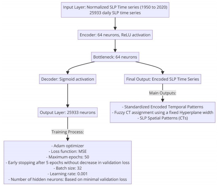
This study presents a novel approach that employs autoencoders (AE)—an artificial neural network—for the nonlinear transformation of time series to a compact latent space for efficient fuzzy clustering. The method was tested on atmospheric sea level pressure (SLP) data towards fuzzy clustering of atmospheric circulation types (CTs). CTs are a group of dates with a similar recurrent SLP spatial pattern. The analysis aimed to explore the effectiveness of AE in producing and improving the characterization of known CTs (i.e., recurrent SLP patterns) derived from traditional linear models like principal component analysis (PCA). After applying both PCA and AE for the linear and nonlinear transformation of the SLP time series, respectively, followed by a fuzzy clustering of the daily SLP time series from each technique, the resulting CTs generated by each method were compared to assess consistency. The findings reveal consistency between the SLP spatial patterns from the two methods, with 58% of the patterns showing congruence matches greater than 0.94. However, when examining the correctly classified dates (i.e., the true positives) using a threshold of 0.8 for the congruence coefficient between the spatial composite map representing the CT and the dates grouped under the CT, AE outperformed PCA with an average improvement of 29.2%. Hence, given AE's flexibility and capacity to model complex nonlinear relationships, this study suggests that AE could be a potent tool for enhancing fuzzy time series clustering, given its capability to facilitate the correct identification of dates when a given CT occurred and assigning the dates to the associated CT.
- fuzzy classification,
- autoencoders,
- principal component analysis,
- sea level pressure,
- artificial neural network
Citation: Chibuike Chiedozie Ibebuchi. Fuzzy time series clustering using autoencoders neural network[J]. AIMS Geosciences, 2024, 10(3): 524-539. doi: 10.3934/geosci.2024027

Related Papers:

Abstract

This study presents a novel approach that employs autoencoders (AE)—an artificial neural network—for the nonlinear transformation of time series to a compact latent space for efficient fuzzy clustering. The method was tested on atmospheric sea level pressure (SLP) data towards fuzzy clustering of atmospheric circulation types (CTs). CTs are a group of dates with a similar recurrent SLP spatial pattern. The analysis aimed to explore the effectiveness of AE in producing and improving the characterization of known CTs (i.e., recurrent SLP patterns) derived from traditional linear models like principal component analysis (PCA). After applying both PCA and AE for the linear and nonlinear transformation of the SLP time series, respectively, followed by a fuzzy clustering of the daily SLP time series from each technique, the resulting CTs generated by each method were compared to assess consistency. The findings reveal consistency between the SLP spatial patterns from the two methods, with 58% of the patterns showing congruence matches greater than 0.94. However, when examining the correctly classified dates (i.e., the true positives) using a threshold of 0.8 for the congruence coefficient between the spatial composite map representing the CT and the dates grouped under the CT, AE outperformed PCA with an average improvement of 29.2%. Hence, given AE's flexibility and capacity to model complex nonlinear relationships, this study suggests that AE could be a potent tool for enhancing fuzzy time series clustering, given its capability to facilitate the correct identification of dates when a given CT occurred and assigning the dates to the associated CT.

References

[1]	Philipp A, Della-Marta PM, Jacobeit J, et al. (2007) Long-term variability of daily North Atlantic–European pressure patterns since 1850 classified by simulated annealing clustering. J Clim 20: 4065–4095. https://doi.org/10.1175/JCLI4175.1 doi: 10.1175/JCLI4175.1
[2]	Pasini A, Lorè M, Ameli F (2006) Neural network modelling for the analysis of forcings/temperatures relationships at different scales in the climate system. Ecol Modell 191: 58–67. https://doi.org/10.1016/j.ecolmodel.2005.08.012 doi: 10.1016/j.ecolmodel.2005.08.012
[3]	Mihailović DT, Mimić G, Arsenić I (2014) Climate predictions: The chaos and complexity in climate models. Adv Meteorol 2014: 878249. https://doi.org/10.1155/2014/878249 doi: 10.1155/2014/878249
[4]	Esteban P, Martin-Vide J, Mases M (2006) Daily atmospheric circulation catalogue for Western Europe using multivariate techniques. Int J Climatol 26: 1501–1515. https://doi.org/10.1002/joc.1391 doi: 10.1002/joc.1391
[5]	Philipp A, Bartholy J, Beck C, et al. (2010) Cost733cat–A database of weather and circulation type classifications. Phys Chem Earth 35: 360–373. https://doi.org/10.1016/j.pce.2009.12.010 doi: 10.1016/j.pce.2009.12.010
[6]	Ibebuchi CC, Richman MB (2023) Circulation typing with fuzzy rotated T-mode principal component analysis: methodological considerations. Theor Appl Climatol, 495–523. https://doi.org/10.1007/s00704-023-04474-5 doi: 10.1007/s00704-023-04474-5
[7]	Huth R, Beck C, Philipp A, et al. (2008) Classifications of atmospheric circulation patterns: recent advances and applications. Ann N Y Acad Sci 1146: 105–152. https://doi.org/10.1196/annals.1446.019 doi: 10.1196/annals.1446.019
[8]	Deligiorgi D, Philippopoulos K, Kouroupetroglou G (2014) An assessment of self-organizing maps and k-means clustering approaches for atmospheric circulation classification. Recent Adv Environ Sci Geosci, 17.
[9]	James G, Witten D, Hastie T, et al. (2013) An introduction to statistical learning. New York: springer. 112: 3–7.
[10]	Hannachi A, Jolliffe IT, Stephenson DB (2007) Empirical orthogonal functions and related techniques in atmospheric science: A review. Int J Climatol 27: 1119–1152.
[11]	Compagnucci RH, Richman MB (2008) Can principal component analysis provide atmospheric circulation or teleconnection patterns? Int J Climatol J R Meteorol Soc 28: 703–726.
[12]	Huth R (2000) A circulation classification scheme applicable in GCM studies. Theor Appl Climatol 67: 1–18. https://doi.org/10.1007/s007040070012 doi: 10.1007/s007040070012
[13]	Chattopadhyay A, Hassanzadeh P, Pasha S (2020) Predicting clustered weather patterns: A test case for applications of convolutional neural networks to spatio-temporal climate data. Sci Rep 10: 1317. https://doi.org/10.1038/s41598-020-57897-9 doi: 10.1038/s41598-020-57897-9
[14]	Davenport FV, Diffenbaugh NS (2021) Using machine learning to analyze physical causes of climate change: A case study of US Midwest extreme precipitation. Geophys Res Lett 48: e2021GL093787. https://doi.org/10.1029/2021GL093787 doi: 10.1029/2021GL093787
[15]	Weyn JA, Durran DR, Caruana R (2020) Improving data-driven global weather prediction using deep convolutional neural networks on a cubed sphere. J Adv Model Earth Sy 12: e2020MS002109. https://doi.org/10.1029/2020MS002109 doi: 10.1029/2020MS002109
[16]	Lee CC, Sheridan SC, Dusek GP, et al. (2023) Atmospheric Pattern–Based Predictions of S2S Sea Level Anomalies for Two Selected US Locations. Artif Intell Earth Syst 2: 220057. https://doi.org/10.1175/AIES-D-22-0057.1 doi: 10.1175/AIES-D-22-0057.1
[17]	Hinton GE, Salakhutdinov RR (2006) Reducing the Dimensionality of Data with Neural Networks. Science 313: 504–507. https://doi.org/10.1126/science.1127647 doi: 10.1126/science.1127647
[18]	Murakami H, Delworth TL, Cooke WF, et al. (2022) Increasing frequency of anomalous precipitation events in Japan detected by a deep learning autoencoder. Earths Future 10: e2021EF002481. https://doi.org/10.1029/2021EF002481 doi: 10.1029/2021EF002481
[19]	Ibebuchi CC, Abu IO, Nyamekye C, et al. (2024) Utilizing Machine Learning to Examine the Spatiotemporal Changes in Africa's Partial Atmospheric Layer Thickness. Sustainability 16: 256. https://doi.org/10.3390/su16010256 doi: 10.3390/su16010256
[20]	Myrzaliyeva M (2022) INVESTIGATING THE IMPACT OF CLIMATE CHANGE ON WEATHER REGIMES USING DIMENSIONALITY REDUCTION WITH DEEP AUTOENCODERS. Available from: https://cris.vub.be/ws/portalfiles/portal/94889169/MA_ACS_Myrzaliyeva_Madina_S3_2122_final.pdf.
[21]	Kurihana T, Franke J, Foster I, et al. (2022) Insight into cloud processes from unsupervised classification with a rotationally invariant autoencoder. arXiv preprint arXiv, 2211.00860. https://doi.org/10.48550/arXiv.2211.00860
[22]	Huang Z, Tan X, Wu X, et al. (2023) Long-Term Changes, Synoptic Behaviors, and Future Projections of Large-Scale Anomalous Precipitation Events in China Detected by a Deep Learning Autoencoder. J Clim 36: 4133–4149. https://doi.org/10.1175/JCLI-D-22-0737.1 doi: 10.1175/JCLI-D-22-0737.1
[23]	Krinitskiy MA, Zyulyaeva YA, Gulev SK (2019) Clustering of polar vortex states using convolutional autoencoders. Available from: https://ceur-ws.org/Vol-2426/paper8.pdf.
[24]	Richard G, Grossin B, Germaine G, et al. (2002) Autoencoder-based time series clustering with energy applications. arXiv preprint arXiv, 2002.03624. https://doi.org/10.48550/arXiv.2002.03624
[25]	Tavakoli N, Siami-Namini S, Adl Khanghah M, et al. (2020) An autoencoder-based deep learning approach for clustering time series data. SN Appl Sci 2: 937. https://doi.org/10.1007/s42452-020-2584-8 doi: 10.1007/s42452-020-2584-8
[26]	Kalinicheva E, Sublime J, Trocan M (2020) Unsupervised satellite image time series clustering using object-based approaches and 3D convolutional autoencoder. Remote Sens 12: 1816. https://doi.org/10.3390/rs12111816 doi: 10.3390/rs12111816
[27]	Harush S, Meidan Y, Shabtai A (2021) DeepStream: autoencoder-based stream temporal clustering and anomaly detection. Comput Secur 106: 102276. https://doi.org/10.1016/j.cose.2021.102276 doi: 10.1016/j.cose.2021.102276
[28]	Noering FKD, Schroeder Y, Jonas K, et al. (2021) Pattern discovery in time series using autoencoder in comparison to nonlearning approaches. Integr Comput-Aid E 28: 237–256. https://doi.org/10.3233/ICA-210650 doi: 10.3233/ICA-210650
[29]	Ibebuchi CC (2021) On the relationship between circulation patterns, the southern annular mode, and rainfall variability in Western Cape. Atmosphere 12: 753. https://doi.org/10.3390/atmos12060753 doi: 10.3390/atmos12060753
[30]	Ibebuchi CC (2021) Circulation pattern controls of wet days and dry days in Free State, South Africa. Meteorol Atmos Phys 133: 1469–1480. https://doi.org/10.1007/s00703-021-00822-0 doi: 10.1007/s00703-021-00822-0
[31]	Hersbach H, Bell B, Berrisford P, et al. (2020) The ERA5 global reanalysis. Q J R Meteorol Soc 146: 1999–2049. https://doi.org/10.1002/qj.3803 doi: 10.1002/qj.3803
[32]	Pedregosa F, Varoquaux G, Gramgort A, et al. (2011). Scikit-learn: Machine learning in Python. J Mach Learn Res 12: 2825–2830.
[33]	Chollet F (2015) Keras. Available from: https://keras.io.
[34]	Glorot X, Bordes A, Bengio Y (2011) Deep sparse rectifier neural networks, Proceedings of the Fourteenth International Conference on Artificial Intelligence and Statistics. JMLR Workshop and Conference Proceedings. 5: 315–323.
[35]	Kingma DP, Ba J (2014) Adam: A method for stochastic optimization. arXiv preprint arXiv, 1412.6980.
[36]	Lorenzo-Seva U, Ten Berge JMF (2006) Tucker's congruence coefficient as a meaningful index of factor similarity. Methodology 2: 57–64. https://doi.org/10.1027/1614-2241.2.2.57 doi: 10.1027/1614-2241.2.2.57
[37]	Gardner MW, Dorling SR (1998) Artificial neural networks (the multilayer perceptron)—a review of applications in the atmospheric sciences. Atmos Environ 32: 2627–2636. https://doi.org/10.1016/S1352-2310(97)00447-0 doi: 10.1016/S1352-2310(97)00447-0
[38]	Campozano L, Mendoza D, Mosquera G, et al. (2020) Wavelet analyses of neural networks-based river discharge decomposition. Hydrol Processes 34: 2302–2312. https://doi.org/10.1002/hyp.13726 doi: 10.1002/hyp.13726
[39]	Castelvecchi D (2016) Can we open the black box of AI? Nat News 538: 20–23.
[40]	Toms BA, Barnes EA, Ebert-Uphoff I (2020) Physically interpretable neural networks for the geosciences: Applications to earth system variability. J Adv Model Earth Sy 12: e2019MS002002. https://doi.org/10.1029/2019MS002002 doi: 10.1029/2019MS002002
[41]	Pierdicca R, Paolanti M (2022) GeoAI: a review of artificial intelligence approaches for the interpretation of complex geomatics data. Geosci Instrum Methods Data Syst 11: 195–218. https://doi.org/10.5194/gi-11-195-2022 doi: 10.5194/gi-11-195-2022
[42]	Mamalakis A, Ebert-Uphoff I, Barnes EA (2020) Explainable artificial intelligence in meteorology and climate science: Model fine-tuning, calibrating trust and learning new science, International Workshop on Extending Explainable AI Beyond Deep Models and Classifiers. Cham: Springer International Publishing. 315–339. https://doi.org/10.1007/978-3-031-04083-2_16
[43]	Labe ZM, Barnes EA (2021) Detecting climate signals using explainable AI with single-forcing large ensembles. J Adv Model Earth Sy 13: e2021MS002464. https://doi.org/10.1029/2021MS002464 doi: 10.1029/2021MS002464
[44]	Karim F, Majumdar S, Darabi H, et al. (2017) LSTM fully convolutional networks for time series classification. IEEE Access 6: 1662–1669. https://doi.org/10.1109/ACCESS.2017.2779939 doi: 10.1109/ACCESS.2017.2779939
[45]	Sadouk L (2019) CNN approaches for time series classification. Time series analysis-data, methods, and applications, 5: 57–78.
[46]	Zhao B, Lu H, Chen S, et al. (2017) Convolutional neural networks for time series classification. J Syst Eng Electron 28: 162–169. https://doi.org/10.21629/JSEE.2017.01.18 doi: 10.21629/JSEE.2017.01.18
[47]	Ibebuchi CC, Richman MB (2024) Deep learning with autoencoders and LSTM for ENSO forecasting. Clim Dyn.

Reader Comments

Your name:*

Email:*
© 2024 the Author(s), licensee AIMS Press. This is an open access article distributed under the terms of the Creative Commons Attribution License (http://creativecommons.org/licenses/by/4.0)