The purpose of this paper is to examine the predictive power of optimistic expectations and satisfaction with life in the country of origin and residence—Bulgaria, over attitudes towards emigration among young Bulgarians with regard to their generational belonging and age differences (i.e. Generation Y or Millennials and Generation Z or Zoomers). Although the correlation between satisfaction with life and migration (attitudes) has been studied in many countries, it has not been examined to date in Bulgaria (a sending, rather than receiving Eastern European country) in the light of optimistic expectations and age differences. Within a cross-sectional survey (N = 1200), representative of young Bulgarians aged 18–35 years—Zoomers aged 18–25 years (N = 444) and Millennials aged 26–35 years (N = 756), carried out in September-October 2021, optimistic expectations for individual development in Bulgaria, satisfaction with life in the country and emigration attitudes were measured using originally designed scales. The findings suggest that the more optimistic expectations about one's own career development and material security in the country are associated with higher satisfaction with life in Bulgaria and reasonably, with more negative attitudes towards emigration. Interestingly, optimistic expectations turned out a stronger antecedent of Zoomers' emigration attitudes compared to those of Millennials and life satisfaction—a stronger predictor of Millennials' emigration attitudes compared to those of Zoomers. Although no significant age differences in life satisfaction were found, Zoomers turned out significantly more optimistic about their future in the country, but also more attuned to emigration compared to Millennials. Young people with previous emigration experience were found to be significantly more likely to emigrate in comparison to those without prior emigration experience. The findings have some important interdisciplinary implications, both for psychological theory and for demographic policy.
Citation: Diana I Bakalova, Ekaterina E Dimitrova. Optimistic expectations and life satisfaction as antecedents of emigration attitudes among Bulgarian Millennials and Zoomers[J]. AIMS Geosciences, 2023, 9(2): 285-310. doi: 10.3934/geosci.2023016
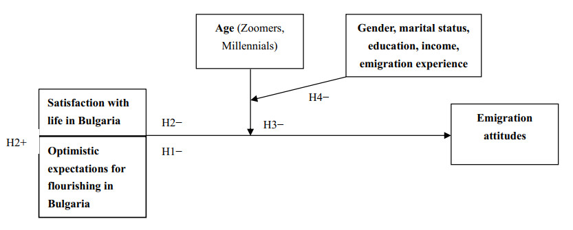
The purpose of this paper is to examine the predictive power of optimistic expectations and satisfaction with life in the country of origin and residence—Bulgaria, over attitudes towards emigration among young Bulgarians with regard to their generational belonging and age differences (i.e. Generation Y or Millennials and Generation Z or Zoomers). Although the correlation between satisfaction with life and migration (attitudes) has been studied in many countries, it has not been examined to date in Bulgaria (a sending, rather than receiving Eastern European country) in the light of optimistic expectations and age differences. Within a cross-sectional survey (N = 1200), representative of young Bulgarians aged 18–35 years—Zoomers aged 18–25 years (N = 444) and Millennials aged 26–35 years (N = 756), carried out in September-October 2021, optimistic expectations for individual development in Bulgaria, satisfaction with life in the country and emigration attitudes were measured using originally designed scales. The findings suggest that the more optimistic expectations about one's own career development and material security in the country are associated with higher satisfaction with life in Bulgaria and reasonably, with more negative attitudes towards emigration. Interestingly, optimistic expectations turned out a stronger antecedent of Zoomers' emigration attitudes compared to those of Millennials and life satisfaction—a stronger predictor of Millennials' emigration attitudes compared to those of Zoomers. Although no significant age differences in life satisfaction were found, Zoomers turned out significantly more optimistic about their future in the country, but also more attuned to emigration compared to Millennials. Young people with previous emigration experience were found to be significantly more likely to emigrate in comparison to those without prior emigration experience. The findings have some important interdisciplinary implications, both for psychological theory and for demographic policy.

| [1] | National Statistical Institute, Demographic and Social Statistics—External Migration Data, 2007–2021. Available from: https://infostat.nsi.bg/infostat/pages/module.jsf?x_2 = 38. |
| [2] |
Borjas GJ (2001) Does Immigration Grease the Wheels of the Labor Market? Brookings Pap Eco Ac 2001: 69–133. https://doi.org/10.1353/eca.2001.0011 doi: 10.1353/eca.2001.0011

|
| [3] |
Ostrachshenko V, Popova O (2014) Life (dis)satisfaction and the intention to migrate: Evidence from Central and Eastern Europe. J Socio-Econ 48: 40–49. http://dx.doi.org/10.1016/j.socec.2013.09.008 doi: 10.1016/j.socec.2013.09.008
|
| [4] |
Cai R, Esipova N, Oppenheimer M, et al. (2014) International migration desires related to subjective well-being. IZA J Migration 3: 8. https://doi.org/10.1186/2193-9039-3-8 doi: 10.1186/2193-9039-3-8
|
| [5] |
Nikolova M, Graham C (2015) In transit: the well-being of migrants from transition and post-transition countries. J Econ Behav Organ 112: 164–186. http://dx.doi.org/10.1016/j.jebo.2015.02.003 doi: 10.1016/j.jebo.2015.02.003
|
| [6] |
Ivlevs A (2014) Happiness and the emigration decision. IZA World Labor 2014: 1–10. https://doi.org/10.15185/izawol.96 doi: 10.15185/izawol.96
|
| [7] |
Ivlevs A (2015) Happy Moves? Assessing the Link Between Life Satisfaction and Emigration Intentions. Int Rev Soc Sci 68: 335–356. https://doi.org/10.1111/kykl.12086 doi: 10.1111/kykl.12086
|
| [8] | Kardas F, Cam Z, Eskisu M, et al. (2019) Gratitude, Hope, Optimism and Life Satisfaction as Predictors of Psychological Well-Being. Eurasian J Educ Res 19: 81–100. |
| [9] | Bekmezci M, ul Rehman W (2023) Immigration of Younger Workers: Generation Z in Turkey, In: Ince F, Ed., Leadership Perspectives on Effective Intergenerational Communication and Management, 150–165. IGI Global. https://doi.org/10.4018/978-1-6684-6140-2.ch009 |
| [10] | European Parliamentary Research Service, Next generation or lost generation? Children, young people and the pandemic, Briefing, 2020. Available from: https://www.europarl.europa.eu/RegData/etudes/BRIE/2020/659404/EPRS_BRI(2020)659404_EN.pdf. |
| [11] | Scholz C (2019) The Generations Z in Europe—An Introduction, Generations Z in Europe (The Changing Context of Managing People), Emerald Publishing Limited, Bingley, 3–31. https://doi.org/10.1108/978-1-78973-491-120191001 |
| [12] | Twenge JM (2015) Time Period and Birth Cohort Differences in Depressive Symptoms in the U.S., 1982–2013. Soc Indic Res 121: 437–454. https://doi.org/10.1007/s11205-014-0647-1 |
| [13] |
Twenge JM, Cooper AB, Joiner TE, et al. (2019) Age, period, and cohort trends in mood disorder indicators and suicide-related outcomes in a nationally representative dataset, 2005–2017. J Abnorm Psychol 128: 185–199. https://doi.org/10.1037/abn0000410 doi: 10.1037/abn0000410
|
| [14] | Khan A, Aleem S, Walia T (2021) Happiness and well-being among generation X, generation Y and generation Z in Indian context: A survey study. Indian J Posit Psychol 12: 70–76. |
| [15] |
Agustina TS, Fauzia DS (2021) The Need For Achievement, Risk-Taking Propensity, And Entrepreneurial Intention Of The Generation Z. Risenologi 6: 96–106. https://doi.org/10.47028/j.risenologi.2021.61.161 doi: 10.47028/j.risenologi.2021.61.161
|
| [16] | Dreyer CH, Stojanová H (2023) How entrepreneurial is German Generation Z vs. Generation Y? A Literature Review. Procedia Comput Sci 217: 155–164. https://doi.org/10.1016/j.procs.2022.12.211 |
| [17] | Dabija DC, Bejan BM, Dinu V (2019) How sustainability oriented is Generation Z in retail? A literature review. Transform Bus Econ 18: 155–164. Available from: http://www.transformations.knf.vu.lt/47/article/hows |
| [18] | Peterson C (2000) The future of optimism. Am Psychol 55: 44–55. |
| [19] |
Tiger L (1985) Ideology as Brain Disease. Zigon J Religion Sci 20: 31–39. https://doi.org/10.1111/j.1467-9744.1985.tb00576.x doi: 10.1111/j.1467-9744.1985.tb00576.x
|
| [20] | Tiger L (1979) Optimism: the biology of hope. Simon & Schuster, New York. |
| [21] | Argyle M (1999) Causes and Correlates of Happiness. In: Kahneman D, Diener E, Schwarz N, (Eds.), Well-Being: The Foundations of Hedonic Psychology, New York: Russell Sage Foundation. 353–373. |
| [22] |
Sharpe J, Martin N, Roth K (2011) Optimism and the Big Five factors of personality: Beyond Neuroticism and Extraversion. Pers Individ Differ 51: 946–951. https://doi.org/10.1016/j.paid.2011.07.033 doi: 10.1016/j.paid.2011.07.033
|
| [23] |
Lench HC (2011) Personality and health outcomes: Making positive expectations a reality. J Happiness Stud 12: 493–507. https://doi.org/10.1007/s10902-010-9212-z doi: 10.1007/s10902-010-9212-z
|
| [24] |
Conversano C, Rotondo A, Lensi E, et al. (2010) Optimism and Its Impact on Mental and Physical Well-Being. Clin Pract Epidemiol Ment Health 6: 25–29. https://doi.org/10.2174/1745017901006010025 doi: 10.2174/1745017901006010025
|
| [25] |
Forgeard M, Seligman M (2012) Seeing the glass half full: A review of the causes and consequences of optimism. Prat Psychol 18: 107–120. https://doi.org/10.1016/j.prps.2012.02.002 doi: 10.1016/j.prps.2012.02.002
|
| [26] |
Peterson C, Seligman M (1987) Explanatory style and illness. J Pers 55: 237–265. https://doi.org/10.1111/j.1467-6494.1987.tb00436.x doi: 10.1111/j.1467-6494.1987.tb00436.x
|
| [27] | Peterson C, Park N, Seligman MEP (2013) Orientations to happiness and life satisfaction: The full life versus the empty life. In: Delle Fave A, Eds., The Exploration of Happiness. Happiness Studies Book Series, Springer, Dordrecht. https://doi.org/10.1007/978-94-007-5702-8_9 |
| [28] |
Kahneman D (2003) Maps of Bounded Rationality: Psychology for Behavioral Economics. Am Econ Rev 93: 1449–1475. https://doi.org/10.1257/000282803322655392 doi: 10.1257/000282803322655392
|
| [29] |
Lench HC, Bench SW (2012) Automatic optimism: Why people assume their futures will be bright. Soc Personal Psychol Compass 6: 347–360. https://doi.org/10.1111/j.1751-9004.2012.00430.x doi: 10.1111/j.1751-9004.2012.00430.x
|
| [30] | Lench HC, Ditto PH (2008) Automatic optimism: Biased use of base rate information for positive and negative events. J Exp Soc Psychol 44: 631–639. https://doi.org/10.1016/j.jesp.2007.02.011 |
| [31] |
Sharot T, Korn CW, Dolan RJ (2011) How unrealistic optimism is maintained in the face of reality. Nat Neurosci 14: 1475–1479. https://doi.org/10.1038/nn.2949 doi: 10.1038/nn.2949
|
| [32] |
McKay R, Dennett D (2009) The evolution of misbelief. Behav Brain Sci 32: 493–510. https://doi.org/10.1017/S0140525X09990975 doi: 10.1017/S0140525X09990975
|
| [33] |
Windschitl PD, Kruger J, Simms E (2003) The Influence of Egocentrism and Focalism on People's Optimism in Competitions: When What Affects Us Equally Affects Me More. J Pers Soc Psychol 85: 389–408. https://doi.org/10.1037/0022-3514.85.3.389 doi: 10.1037/0022-3514.85.3.389
|
| [34] |
Loewenstein GF, Weber EU, Hsee CK (2001) Risk as Feelings. Psychol Bull 127: 267–286. https://doi.org/10.1037//0033-2909.127.2.267 doi: 10.1037//0033-2909.127.2.267
|
| [35] | Aspinwall LG, Taylor SE (1992) Modeling cognitive adaptation: A longitudinal investigation of the impact of individual differences and coping on college adjustment and performance. J Pers Soc Psychol 63: 989–1003. https://doi.org/10.1037/0022-3514.63.6.989 |
| [36] | Argyle M (1986) The psychology of happiness, London: Methuen. https://doi.org/10.4324/9781315812212 |
| [37] |
Diener D, Emmons RA, Larsen RJ, et al. (1985) The satisfaction with life scale. J Pers Assess 49: 71–75. https://doi.org/10.1207/s15327752jpa4901_13 doi: 10.1207/s15327752jpa4901_13
|
| [38] | Diener E, Lucas R, Oishi S (2002) Subjective well-being: The science of happiness and life satisfaction. The handbook of positive psychology, New York, Oxford University Press. 63–73. Available from: https://greatergood.berkeley.edu/images/uploads/Diener-Subjective_Well-Being.pdf. |
| [39] |
Veenhoven R (1996) Happy life-expectancy. Soc Indic Res 39: 1–58. https://doi.org/10.1007/BF00300831 doi: 10.1007/BF00300831
|
| [40] | Bakalova D, Bakracheva M, Mizova B (2015) Happiness and life satisfaction: In Search for Ourselves, Sofia, Colbis. Available from: https://www.researchgate.net/publication/338220961_SASTIE_I_UDOVLETVORENOST_OT_ZIVOTA_V_TRSENE_NA_PTA_KM_SEBE_SI. |
| [41] |
Baltacı A, Yağlı N (2020) Optimism, happiness, life meaning and life satisfaction levels of the faculty of divinity students: A multi-sample correlational study. Spiritual Psychol Couns 5: 167–184. https://doi.org/10.37898/spc.2020.5.2.91 doi: 10.37898/spc.2020.5.2.91
|
| [42] |
Brief AP, Butcher AH, George JM, et al. (1993) Integrating bottom-up and top-down theories of subjective well-being: The case of health. J Pers Soc Psychol 64: 646–653. https://doi.org/10.1037/0022-3514.64.4.646 doi: 10.1037/0022-3514.64.4.646
|
| [43] |
Lee ES (1966) A theory of migration. Demography 3: 47–57. https://doi.org/10.2307/2060063 doi: 10.2307/2060063
|
| [44] | Toney MB, Bailey AK (2014) Migration, an Overview. Encyclopedia of Quality of Life and Well-Being Research, Springer, Dordrecht. 4044–4050. https://doi.org/10.1007/978-94-007-0753-5_1804 |
| [45] | Ellis A, Harper RA (1961) A new guide to rational living, Prentice-Hall. Available from: https://www.academia.edu/33893248/3_i_t_ew_Guide_to_Rational_Living. |
| [46] | Rosenberg M, Hovland I (1960) Cognitive, affective, and behavioral components of attitudes. In: Hovland C, Rosenberg J, Eds., Attitude organization and change, New Haven, CT, Yale University Press. 1–14. |
| [47] | Rokeach M (1968) Beliefs, Attitudes and Values: A Theory of Organization and Change, San Francisco, Jossey-Bass. |
| [48] | Pickens J (2005) Attitudes and perceptions. Organizational behavior in health care, 43–76. |
| [49] |
Schwarz N (2007) Attitude Construction: Evaluation in Context. Social Cognit 25: 638–656. https://doi.org/10.1521/soco.2007.25.5.638 doi: 10.1521/soco.2007.25.5.638
|
| [50] | IOM's Global Migration Data Analysis Center, Measuring Global Migration Potential, 2010–2015, 2017. Available from: https://publications.iom.int/books/global-migration-data-analysis-centre-data-briefing-series-issue-no-9-july-2017?utm_source = link_newsv9 & utm_campaign = item_245216 & utm_medium = copy |
| [51] | Eagly A, Chaiken S (1993) The psychology of attitudes, Harcourt Brace Jovanovich College Publishers. |
| [52] | Chaiklin H (2011) Attitudes, behavior, and social practice. J Sociol Soc Welfare 38: 31–54. |
| [53] | Ajzen I (1980) Understanding attitudes and predicting social behavior, Prentice-Hall. |
| [54] | Ajzen I, Fishbein M (2005) The influence of attitudes on behavior. In: Albarracin D, Johnson BT, Zanna MP Eds., The Handbook of Attitudes, Mahwah, NJ, Lawrence Erlbaum Associates. 173–221. https://doi.org/10.4324/9781410612823 |
| [55] | Мirchev М (2011) Texts—invitation to sociology. Sofia, АSSА-М. |
| [56] | Helliwell J, Richard L, Sachs J (2013) World happiness report. New York, UN Sustainable Development Solutions Network. Available from: https://worldhappiness.report/ed/2013/ |
| [57] |
Oswald A, Proto E, Sgroi D (2015) Happiness and productivity. J Labor Econ 33: 789–822. https://doi.org/10.1086/681096 doi: 10.1086/681096
|
| [58] |
Akay A, Constant A, Giulietti C (2014) The impact of immigration on the wellbeing of natives. J Econ Behav Organ 103: 72–92. https://doi.org/10.1016/j.jebo.2014.03.024 doi: 10.1016/j.jebo.2014.03.024
|
| [59] |
Diener E, Chan M (2011) Happy people live longer: Subjective well-being contributes to health and longevity. Applied Psychology: Health Well-Being 3: 1–43. https://doi.org/10.1111/j.1758-0854.2010.01045.x doi: 10.1111/j.1758-0854.2010.01045.x
|
| [60] | De Neve J, Diener E, Tay L, et al. (2013) The Objective Benefits of Subjective Well-Being, World Happiness Report 2013, New York, UN Sustainable Development Solutions Network. Morocco, 1–35. Available from: https://EconPapers.repec.org/RePEc:ehl:lserod:51669 |
| [61] | Graham C, Markowitz J (2011) Aspirations and Happiness of Potential Latin American Immigrants. J Soc Res Policy 2: 9–25. https://www.researchgate.net/publication/285642914 |
| [62] |
Chindarkar N (2014) Is Subjective Well-Being of Concern to Potential Migrants from Latin America? Soc Indic Res 115: 159–182. https://doi.org/10.1007/s11205-012-0213-7 doi: 10.1007/s11205-012-0213-7
|
| [63] |
Polgreen LA, Simpson NB (2011) Happiness and International Migration. J Happiness Stud 12: 819–840. https://doi.org/10.1007/s10902-010-9229-3 doi: 10.1007/s10902-010-9229-3
|
| [64] |
De Jong GF (2000) Expectations, gender, and norms in migration decision making. Popul Stud 54: 307–319. https://doi.org/10.1080/713779089 doi: 10.1080/713779089
|
| [65] |
Burda MC, Härdle W, Müller M, et al. (1998) Semiparametric Analysis of German East-West Migration Intentions: Facts and Theory. J Appl Economet 13: 525–541. https://doi.org/10.1002/(SICI)1099-1255(1998090)13:5<525::AID-JAE508>3.0.CO;2-C doi: 10.1002/(SICI)1099-1255(1998090)13:5<525::AID-JAE508>3.0.CO;2-C
|
| [66] |
Van Dalen HP, Henkens K (2013) Explaining emigration intentions and behaviour in the Netherlands, 2005–10. Popul Stud 67: 225–241. https://doi.org/10.1080/00324728.2012.725135 doi: 10.1080/00324728.2012.725135
|
| [67] |
Ek E, Koiranena M, Raatikkaa VP, et al. (2008) Psychosocial factors as mediators between migration and subjective well-being among young Finnish adults. Soc Sci Med 66: 1545–1556. https://doi.org/10.1016/j.socscimed.2007.12.018 doi: 10.1016/j.socscimed.2007.12.018
|
| [68] |
Boneva B, Frieze I (2001) Toward a Concept of Migrant Personality. J Soc Issues 57: 477–491. https://doi.org/10.1111/0022-4537.00224 doi: 10.1111/0022-4537.00224
|
| [69] |
Nowok B, Van Ham M, Findlay A, et al. (2013) Does migration make you happy? A longitudinal study of internal migration and subjective well-being. Environ Plann A 45: 986–1002. https://doi.org/10.1068/a45287 doi: 10.1068/a45287
|
Figures(1) / Tables(9)

Diana I Bakalova, Ekaterina E Dimitrova. Optimistic expectations and life satisfaction as antecedents of emigration attitudes among Bulgarian Millennials and Zoomers[J]. AIMS Geosciences, 2023, 9(2): 285-310. doi: 10.3934/geosci.2023016


 DownLoad: