Numerical modelling of a deep closed-loop geothermal system: evaluating the Eavor-Loop

Joseph J. Kelly; Christopher I. McDermott; Joseph J. Kelly; Christopher I. McDermott

doi:10.3934/geosci.2022011

AIMS Geosciences

2022, Volume 8, Issue 2: 175-212. doi: 10.3934/geosci.2022011

Previous Article Next Article

Research article

Numerical modelling of a deep closed-loop geothermal system: evaluating the Eavor-Loop

School of GeoSciences, The University of Edinburgh, Edinburgh, UK

Received: 29 November 2021 Revised: 18 January 2022 Accepted: 09 February 2022 Published: 23 February 2022

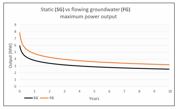
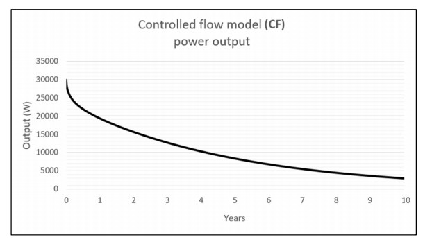
Conventional geothermal energy systems are limited by hydrogeological conditions and environmental risks, and wind/solar solutions have issues with intermittency and the need for grid storage. Deep closed-loop geothermal systems such as the Eavor-Loop are championed as scalable, dispatchable, zero-emission alternative energy technologies, but as yet they are largely untested. A series of numerical models are created using the finite element method to evaluate the power output claims made by Eavor. The models use typical parameter values to create a simplified study domain. The modelling results show that the power output claims are plausible, although the upper range of their predictions would likely require production temperatures in excess of 150 ℃. The technology is shown to be scalable by adding additional lateral wellbore arrays, but this leads to a reduction in efficiency due to thermal interference. It is demonstrated that the presence of groundwater can improve power output at relatively high hydraulic conductivity values. Doubt is cast on the likelihood of finding such values in the deep subsurface. Flow rate is shown to increase power output, but the practicality of using it to follow energy demand is not established. Various limitations of the study are discussed, and suggestions are made for future work which could fill in the remaining knowledge gaps.
- deep closed-loop geothermal,
- heat transport,
- numerical modelling,
- baseload power,
- multilaterals
Citation: Joseph J. Kelly, Christopher I. McDermott. Numerical modelling of a deep closed-loop geothermal system: evaluating the Eavor-Loop[J]. AIMS Geosciences, 2022, 8(2): 175-212. doi: 10.3934/geosci.2022011

Related Papers:

Abstract

Conventional geothermal energy systems are limited by hydrogeological conditions and environmental risks, and wind/solar solutions have issues with intermittency and the need for grid storage. Deep closed-loop geothermal systems such as the Eavor-Loop are championed as scalable, dispatchable, zero-emission alternative energy technologies, but as yet they are largely untested. A series of numerical models are created using the finite element method to evaluate the power output claims made by Eavor. The models use typical parameter values to create a simplified study domain. The modelling results show that the power output claims are plausible, although the upper range of their predictions would likely require production temperatures in excess of 150 ℃. The technology is shown to be scalable by adding additional lateral wellbore arrays, but this leads to a reduction in efficiency due to thermal interference. It is demonstrated that the presence of groundwater can improve power output at relatively high hydraulic conductivity values. Doubt is cast on the likelihood of finding such values in the deep subsurface. Flow rate is shown to increase power output, but the practicality of using it to follow energy demand is not established. Various limitations of the study are discussed, and suggestions are made for future work which could fill in the remaining knowledge gaps.

References

[1]	Falcone G, Liu X, Okech RR, et al. (2018) Assessment of deep geothermal energy exploitation methods: the need for novel single-well solutions. Energy 160: 54-63. https://doi.org/10.1016/j.energy.2018.06.144 doi: 10.1016/j.energy.2018.06.144
[2]	Schulz SU (2008) Investigations on the improvement of the energy output of a closed loop geothermal system (CLGS). Technischen Universität Berlin, Germany. Available from: https://www.osti.gov/etdeweb/biblio/21240869.
[3]	van Oort E, Chen D, Ashok P, et al. (2021) Constructing deep closed-loop geothermal wells for globally scalable energy production by leveraging oil and gas ERD and HPHT well construction expertise. In SPE/IADC International Drilling Conference and exhibition, Virtual, SPE-204097-MS. https://doi.org/10.2118/204097-MS
[4]	Wang G, Song X, Shi Y, et al. (2020) Comparison of production characteristics of various coaxial closed-loop geothermal systems. Energy Convers Manage 225: 113437. https://doi.org/10.1016/j.enconman.2020.113437 doi: 10.1016/j.enconman.2020.113437
[5]	Gluyas JG, Adams CA, Busby JP, et al. (2018) Keeping warm: a review of deep geothermal potential of the UK. Proc Inst Mech Eng Part A 232: 115-126. https://doi.org/10.1177/0957650917749693 doi: 10.1177/0957650917749693
[6]	Geiser P, Marsh B, Hilpert M (2016) Geothermal: The marginalization of Earth's largest and greenest energy source. In Proceedings, 43rd Workshop on Geothermal Reservoir Engineering, Stanford University, Stanford, CA. Available from: https://www.researchgate.net/publication/297471727.
[7]	Scherer JA, Higgins B, Muiret JR, et al. (2020) California Energy Commission consultant report: Closed-loop geothermal demonstration project, confirming models for large-scale closed-loop geothermal projects in California. Greenfire Energy Inc. Available from: https://www.energy.ca.gov/sites/default/files/2021-05/CEC-300-2020-007.pdf.
[8]	Sångfors B (2021) Re: Efficiency of Organic Rankine Cycle? Available from: https://www.researchgate.net/post/Efficiency_of_Organic_Rankine_Cycle.
[9]	Van Horn A, Amaya A, Higgins B, et al. (2020) New opportunities and applications for closed-loop geothermal energy systems. GRC Trans 44: 1123-1143.
[10]	Matuszewska D, Kuta M, Górski J (2019) The environmental impact of renewable energy technologies shown in cases of ORC-Based Geothermal Power Plant. In 2019 IOP Conf. Ser.: Earth & Environ. Sci., 214: 012142. https://doi.org/10.1088/1755-1315/214/1/012142
[11]	Vany J, Hirschmiller J, Toews M (2020) Subsurface characterization methods for multilateral closed loop geothermal systems. Case study of field scale technology demonstration project in Alberta, Canada. GeoConvention 2020. Available from: https://geoconvention.com/wp-content/uploads/abstracts/2020/57874-subsurface-characterization-methods-for-multilater.pdf.
[12]	Fallah AH, Gu Q, Chen D, et al. (2021) Globally scalable geothermal energy production through managed pressure operation control of deep closed-loop well systems. Energy Convers Manage 236: 114056. https://doi.org/10.1016/j.enconman.2021.114056 doi: 10.1016/j.enconman.2021.114056
[13]	Collins L (2021) Oil giants BP and Shell become part-owners of 'world-changing' deep geothermal innovator Eavor. Available from: https://www.rechargenews.com/2-1-963275.
[14]	Eavor Media Kit 15 (2021) Eavor Technologies Inc. Available from: https://www.eavor.com/mediakit/.
[15]	Oldenburg C, Pan L, Muir M, et al. (2016) Numerical simulation of critical factors controlling heat extraction from geothermal systems using a closed-loop heat exchange method. In Proceedings, 41^st Workshop on Geothermal Reservoir Engineering, Stanford University. Available from: https://pangea.stanford.edu/ERE/pdf/IGAstandard/SGW/2016/Oldenburg2.pdf.
[16]	Wang G, Song X, Shi Y, et al. (2021) Heat extraction analysis of a novel multilateral-well coaxial closed-loop geothermal system. Renewable Energy 163: 974-986. https://doi.org/10.1016/j.renene.2020.08.121 doi: 10.1016/j.renene.2020.08.121
[17]	Collins L (2020) Unlimited, on-demand renewable energy anywhere in the world-is Eavor-Loop climate change's holy grail? Available from: https://www.rechargenews.com/transition/2-1-901385.
[18]	Yuan W, Chen Z, Grasby SE, et al. (2021) Closed-loop geothermal energy recovery from deep high enthalpy systems, Renewable Energy 177: 976-991. https://doi.org/10.1016/j.renene.2021.06.028 doi: 10.1016/j.renene.2021.06.028
[19]	McClure M (2021) Why deep closed-loop geothermal is guaranteed to fail. Available from: https://www.resfrac.com/blog/why-deep-closed-loop-geothermal-guaranteed-fail.
[20]	Tolooiyan A, Hemmingway P (2014) A preliminary study of the effect of groundwater flow on the thermal front created by borehole heat exchangers. Int J Low-Carbon Technol 9: 284-295. https://doi.org/10.1093/ijlct/cts077 doi: 10.1093/ijlct/cts077
[21]	Wu B, Ma T, Feng G, et al. (2017) An approximate solution for predicting the heat extraction and preventing the loss from a closed-loop geothermal reservoir. Geofluids 2017: 2041072. https://doi.org/10.1155/2017/2041072 doi: 10.1155/2017/2041072
[22]	Chen C, Cai W, Naumov D, et al. (2021) Numerical investigation on the capacity and efficiency of a deep enhanced U-tube borehole heat exchanger system for building heating. Renewable Energy 169: 557-572. https://doi.org/10.1016/j.renene.2021.01.033 doi: 10.1016/j.renene.2021.01.033
[23]	Shao H, Hein P, Sachse A, et al. (2016) Geoenergy modelling Ⅱ, shallow geothermal systems. Springer Briefs in Energy, ISSN 2191-5539. https://doi.org/10.1007/978-3-319-45057-5
[24]	Böttcher N, Watanabe N, Kolditz O (2015) OpenGeoSys tutorial, Basics of heat transport processes in geothermal systems. Springer Briefs in Energy, via opengeosys.org. Available from: https://ogsstorage.blob.core.windows.net/web/Books/Geoenergy-Model-I/Basics-of-Heat-Transport-Processes-in-Geothermal-Systems-opt.pdf.
[25]	McDermott CI, Randriamanjatosoa ARL, Tenzer H, et al. (2006) Simulation of heat extraction from crystalline rocks: The influence of coupled processes of differential reservoir cooling. Geothermics 35: 321-344. https://doi.org/10.1016/j.geothermics.2006.05.002 doi: 10.1016/j.geothermics.2006.05.002
[26]	Kolditz O (2002) Computational Methods in Environmental Fluid Mechanics. Springer-Verlag, Berlin, 378. https://doi.org/10.1007/978-3-662-04761-3
[27]	Wagner W, Kruse A (1998) Properties of Water and Steam: The Industrial Standard IAPWS-IF97 for the Thermodynamic Properties and Supplementary Equations for Other Properties. Springer, Berlin, 354. Available from: http://www.worldcat.org/oclc/1124445727.
[28]	Chapman DS (1986) Thermal gradients in the continental crust. Geological Society, London, Special Publications, 24: 63-70. https://doi.org/10.1144/GSL.SP.1986.024.01.07 doi: 10.1144/GSL.SP.1986.024.01.07
[29]	Freeze RA, Cherry JA (1979) Groundwater. Prentice-Hall, Englewood Cliffs, NJ, 29. Available from: http://hydrogeologistswithoutborders.org/wordpress/1979-toc/.
[30]	Kuang X, Jiao JJ (2014) An integrated permeability-depth model for Earth's crust. Geophys Res Lett 41: 7539-7545. doi.org/10.1002/2014GL061999

Reader Comments

Your name:*

Email:*
© 2022 the Author(s), licensee AIMS Press. This is an open access article distributed under the terms of the Creative Commons Attribution License (http://creativecommons.org/licenses/by/4.0)