Artificial neural network based PERSIANN data sets in evaluation of hydrologic utility of precipitation estimations in a tropical watershed of Sri Lanka

Miyuru B Gunathilake; Thamashi Senerath; Upaka Rathnayake; Miyuru B Gunathilake; Thamashi Senerath; Upaka Rathnayake

doi:10.3934/geosci.2021027

AIMS Geosciences

2021, Volume 7, Issue 3: 478-489. doi: 10.3934/geosci.2021027

Previous Article Next Article

Research article

Artificial neural network based PERSIANN data sets in evaluation of hydrologic utility of precipitation estimations in a tropical watershed of Sri Lanka

1.
Department of Civil Engineering, Faculty of Engineering, Sri Lanka Institute of Information Technology (SLIIT), Malabe, Sri Lanka
2.
Central Engineering Services (Pvt) Limited, Bauddhaloka Mawatha, Colombo 7, Sri Lanka

Received: 01 June 2021 Accepted: 31 August 2021 Published: 06 September 2021

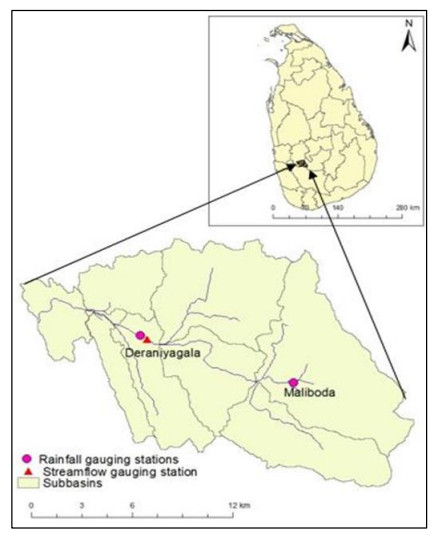
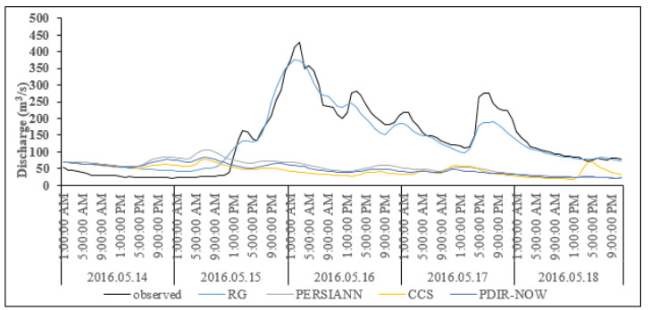
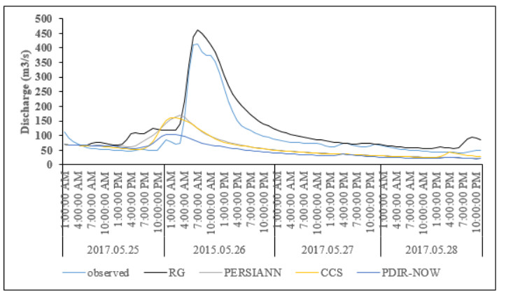
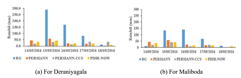
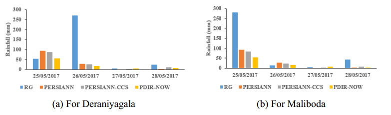
The developments of satellite technologies and remote sensing (RS) have provided a way forward with potential for tremendous progress in estimating precipitation in many regions of the world. These products are especially useful in developing countries and regions, where ground-based rain gauge (RG) networks are either sparse or do not exist. In the present study the hydrologic utility of three satellite-based precipitation products (SbPPs) namely, Precipitation Estimation from Remotely Sensed Information using Artificial Neural Networks (PERSIANN), PERSIANN-Cloud Classification System (PERSIANN-CCS) and Precipitation Estimation from Remotely Sensed Information using Artificial Neural Networks-Dynamic Infrared Rain Rate near real-time (PDIR-NOW) were examined by using them to drive the Hydrologic Engineering Center-Hydrologic Modeling System (HEC-HMS) hydrologic model for the Seethawaka watershed, a sub-basin of the Kelani River Basin of Sri Lanka. The hydrologic utility of SbPPs was examined by comparing the outputs of this modelling exercise against observed discharge records at the Deraniyagala streamflow gauging station during two extreme rainfall events from 2016 and 2017. The observed discharges were simulated considerably better by the model when RG data was used to drive it than when these SbPPs. The results demonstrated that PERSIANN family of precipitation products are not capable of producing peak discharges and timing of peaks essential for near-real time flood-forecasting applications in the Seethawaka watershed. The difference in performance is quantified using the Nash-Sutcliffe Efficiency, which was > 0.80 for the model when driven by RGs, and < 0.08 when driven by the SbPPs. Amongst the SbPPs, PERSIANN performed best. The outcomes of this study will provide useful insights and recommendations for future research expected to be carried out in the Seethawaka watershed using SbPPs. The results of this study calls for the refinement of retrieval algorithms in rainfall estimation techniques of PERSIANN family of rainfall products for the tropical region.
- discharge,
- PERSIANN,
- rainfall,
- seethawaka watershed
Citation: Miyuru B Gunathilake, Thamashi Senerath, Upaka Rathnayake. Artificial neural network based PERSIANN data sets in evaluation of hydrologic utility of precipitation estimations in a tropical watershed of Sri Lanka[J]. AIMS Geosciences, 2021, 7(3): 478-489. doi: 10.3934/geosci.2021027

Related Papers:

Abstract

The developments of satellite technologies and remote sensing (RS) have provided a way forward with potential for tremendous progress in estimating precipitation in many regions of the world. These products are especially useful in developing countries and regions, where ground-based rain gauge (RG) networks are either sparse or do not exist. In the present study the hydrologic utility of three satellite-based precipitation products (SbPPs) namely, Precipitation Estimation from Remotely Sensed Information using Artificial Neural Networks (PERSIANN), PERSIANN-Cloud Classification System (PERSIANN-CCS) and Precipitation Estimation from Remotely Sensed Information using Artificial Neural Networks-Dynamic Infrared Rain Rate near real-time (PDIR-NOW) were examined by using them to drive the Hydrologic Engineering Center-Hydrologic Modeling System (HEC-HMS) hydrologic model for the Seethawaka watershed, a sub-basin of the Kelani River Basin of Sri Lanka. The hydrologic utility of SbPPs was examined by comparing the outputs of this modelling exercise against observed discharge records at the Deraniyagala streamflow gauging station during two extreme rainfall events from 2016 and 2017. The observed discharges were simulated considerably better by the model when RG data was used to drive it than when these SbPPs. The results demonstrated that PERSIANN family of precipitation products are not capable of producing peak discharges and timing of peaks essential for near-real time flood-forecasting applications in the Seethawaka watershed. The difference in performance is quantified using the Nash-Sutcliffe Efficiency, which was > 0.80 for the model when driven by RGs, and < 0.08 when driven by the SbPPs. Amongst the SbPPs, PERSIANN performed best. The outcomes of this study will provide useful insights and recommendations for future research expected to be carried out in the Seethawaka watershed using SbPPs. The results of this study calls for the refinement of retrieval algorithms in rainfall estimation techniques of PERSIANN family of rainfall products for the tropical region.

References

[1]	Roca R, Alexander LV, Potter G, et al. (2019) FROGS: A daily 1° × 1° gridded precipitation database of rain gauge, satellite and reanalysis products. Earth Syst Sci Data 11: 1017-1035. doi: 10.5194/essd-11-1017-2019
[2]	Krajewski WF, Ciach GJ, Habib E (2003) An analysis of small-scale rainfall variability in different climatic regimes. Hydrol Sci J 48: 151-162. doi: 10.1623/hysj.48.2.151.44694
[3]	Lakshmi V, Fayne J, Bolten J (2018) A comparative study of available water in the major river basins of the world. J Hydrol 567: 510-532. doi: 10.1016/j.jhydrol.2018.10.038
[4]	Ayoub AB, Tangang F, Juneng L, et al. (2020) Evaluation of Gridded Precipitation Datasets in Malaysia. Remote Sens 12: 1-22. doi: 10.3390/rs12040613
[5]	Joyce RJ, Janowiak JE, Arkin PA, et al. (2004) CMORPH: A Method that Produces Global Precipitation Estimates from Passive Microwave and Infrared Data at High Spatial and Temporal Resolution. J Hydrometeorol 5: 487-503. doi: 10.1175/1525-7541(2004)005<0487:CAMTPG>2.0.CO;2
[6]	Sorooshian S, Hsu K, Gao X, et al. (2000) Evaluation of PERSIANN system satellite-based estimates of tropical rainfall. Bull Am Meteorol Soc 81: 2035-2046. doi: 10.1175/1520-0477(2000)081<2035:EOPSSE>2.3.CO;2
[7]	Huffman GJ, Bolvin DT, Nelkin EJ, et al. (2007) The TRMM multi-satellite precipitation analysis (TMPA): quasi-global, multiyear, combined-sensor precipitation estimates at fine scales. J Hydrometeorol 8: 38-55. doi: 10.1175/JHM560.1
[8]	Beck HE, Wood EF, Pan M, et al. (2019) MSWEP V2 Global 3-Hourly 0.1° Precipitation: Methodology and Quantitative Assessment. Bull Am Meteorol Soc 100: 473-500. doi: 10.1175/BAMS-D-17-0138.1
[9]	Funk C, Peterson P, Landsfeld M, et al. (2015) The climate hazards infrared precipitation with stations-a new environmental record for monitoring extremes. Sci Data 2: 150066. doi: 10.1038/sdata.2015.66
[10]	Maidment RI, Grimes D, Black E, et al. (2017) A new, long-term daily satellite-based rainfall dataset for operational monitoring in Africa. Sci Data 4: 170063. doi: 10.1038/sdata.2017.63
[11]	Vila DA, De Goncalves LGG, Toll DL, et al. (2009) Statistical Evaluation of Combined Daily Gauge Observations and Rainfall Satellite Estimates over Continental South American. J Hydrometeorol 10: 533-543. doi: 10.1175/2008JHM1048.1
[12]	Dinku T, Connor SJ, Ceccato P (2010) Comparison of CMORPH and TRMM-3B42 over Mountainous Regions of Africa and South America, Satellite Rainfall Applications for Surface Hydrology, Springer, Dordrecht, 193-204.
[13]	Bitew MM, Gebremichael M, Ghebremichael LT, et al. (2012) Evaluation of High-Resolution Satellite Rainfall Products through Streamflow Simulation in a Hydrological Modeling of a Small Mountainous Watershed in Ethiopia. J Hydrometeorol 13: 338-350. doi: 10.1175/2011JHM1292.1
[14]	Alazzy AA, Lü H, Chen R, et al. (2017) Evaluation of satellite precipitation products and their potential influence on hydrological modeling over the Ganz river basin of the Tibetan plateau. Adv Meteorol 2017: 1-23. doi: 10.1155/2017/3695285
[15]	Bui HT, Ishidaira H, Shaowei N (2019) Evaluation of the use of global satellite-gauge and satellite-only precipitation products in stream flow simulations. Appl Water Sci 9: 53. doi: 10.1007/s13201-019-0931-y
[16]	Nashwan MS, Shahid S, Dewan A, et al. (2020) Performance of five high resolution satellite-based precipitation products in arid region of Egypt: An evaluation. Atmos Res 236: 104809. doi: 10.1016/j.atmosres.2019.104809
[17]	Salehie O, Ismail T, Shahid S, et al. (2021) Ranking of gridded precipitation datasets by merging compromise programming and global performance index: a case study of the Amu Darya basin. Theor Appl Climatol 144: 985-999. doi: 10.1007/s00704-021-03582-4
[18]	Zhang T, Yang Y, Dong Z, et al. (2021) Multiscale Assessment of Three Satellite Precipitation Products (TRMM, CMORPH, and PERSIANN) in the Three Gorges Reservoir Area in China. Adv Meteorol 2021: 1-27.
[19]	Yoshimoto S, Amarnath G (2017) Applications of Satellite-Based Rainfall Estimates in Flood Inundation Modeling-A Case Study in Mundeni Aru River Basin, Sri Lanka. Remote Sens 9: 998. doi: 10.3390/rs9100998
[20]	Gunathilake MB, Karunanayake C, Gunathilake AS, et al. (2021) Hydrological models and Artificial Neural Networks (ANNs) to simulate streamflow in a tropical catchment of Sri Lanka. Appl Comput Intell Soft Comput 6683389: 1-9.
[21]	De Silva MMGT, Weerakoon SB, Herath S (2014) Modeling of Event and Continuous Flow Hydrographs with HEC-HMS: Case Study in the Kelani River Basin, Sri Lanka. J Hydrologic Engineering 19: 800-806. doi: 10.1061/(ASCE)HE.1943-5584.0000846
[22]	Jayadeera PM, Wijesekera NTS (2019) A Diagnostic Application of HEC-HMS Model to Evaluate the Potential for Water Management in the Ratnapura Watershed of Kalu Ganga Sri Lanka. Eng J Inst Eng Sri Lanka 52: 11-21.
[23]	Khaniya B, Wanniarachchi S, Rathnayake U (2017) Importance of hydrologic simulation for LIDs and BMPs design using HEC-HMS: A case demonstration. Int J Hydro 1: 138-146.
[24]	Rajendran M, Gunawardena ERN, Dayawansa NDK (2020) Runoff Prediction in an Ungauged Catchment of Upper Deduru-Oya Basin, Sri Lanka: A Comparison of HEC-HMS and WEAP Models. Int J Prog Sci Technol 18: 121-129.
[25]	Perera KTN, Wijayaratna TMN, Jayatillake HM, et al. (2020) Hydrological principle behind the development of series of bunds in ancient tank cascades in small catchments, Sri Lanka. Water Pract Technol 15: 1174-1189. doi: 10.2166/wpt.2020.088
[26]	Munasinghe DSN, Najim MMM, Quadroni S, et al. (2021) Impacts of streamflow alteration on benthic macroinvertebrates by mini-hydro diversion in Sri Lanka. Sci Rep 11: 546. doi: 10.1038/s41598-020-79576-5
[27]	Gunathilake MB, Panditharathne P, Gunathilake AS, et al. (2020) Application of a HEC-HMS model on event-based simulations in a tropical watershed. Eng Appl Sci Res 47: 349-360.
[28]	Goonathilake SA, Perera N, Silva GD, et al. (2016) Natural resources profile: medium to long-term multi-stakeholder strategy and action plan for management and conservation of the Kelani River Basin 2016-2020. Colombo, International Union for Conservation of Nature Sri-Lanka Country Office and Central Environmental Authority, Sri Lanka, 1-36.
[29]	Department of Meteorology. 2016. Available from: http://www.meteo.gov.lk/index.php?option=com_content&view=article&id=94&Itemid=310&lang=en&lang=en).
[30]	Bastiaanssen WGM, Chandrapala L (2003) Water balance variability across Sri Lanka for assessing agricultural and environmental water use. Agric Water Manage 58: 171-192. doi: 10.1016/S0378-3774(02)00128-2
[31]	FAO ⅡASA. Harmonized World Soil Database, 2012. Available from: http://www.fao.org/soils-portal/data-hub/soil-maps-and-databases/harmonized-world-soil-database-v12/en/.
[32]	Moriasi D, Arnold J, Van Liew M, et al. (2007) Model Evaluation Guidelines for Systematic Quantification of Accuracy in Watershed Simulations. Trans ASABE 50: 885-900 doi: 10.13031/2013.23153
[33]	Behrangi A, Andreadis K, Fisher JB, et al. (2014) Satellite-based Precipitation Estimation and Its Application for Streamflow Prediction over Mountainous Western U.S. Basins. J Appl Meteorol Climatol 53: 2823-2842. doi: 10.1175/JAMC-D-14-0056.1
[34]	Gunathilake MB, Amaratunga V, Perera A, et al. (2020) Statistical evaluation and hydrologic simulation capacity of different satellite-based precipitation products (SbPPs) in the Upper Nan River Basin, Northern Thailand. J Hydrol Reg Stud 32: 1-16.
[35]	Bitew MM, Gebremichael M (2010) Evaluation through independent measurements: Complex terrain and humid tropical region in Ethiopia, Satellite Rainfall Applications for Surface Hydrology. Springer, Dordrecht, 205-214.
[36]	Hong Y, Gochis D, Cheng JT, et al. (2007) Evaluation of PERSIANN-CCS rainfall measurement using the NAME Event Rain Gauge Network. J Hydrometeorol 8: 469-482. doi: 10.1175/JHM574.1
[37]	Gao YC, Liu MF (2013) Evaluation of high-resolution satellite precipitation products using rain gauge observations over the Tibetan Plateau. Hydrol Earth Syst Sci 17: 837-849. doi: 10.5194/hess-17-837-2013
[38]	Nguyen P, Thorstensen A, Sorooshian S, et al. (2015) Flood forecasting and inundation mapping using HiResFlood-UCI and near-real-time satellite precipitation data: the 2008 Iowa flood. J Hydrometeorol 16: 1171-1183, doi: 10.1175/JHM-D-14-0212.1
[39]	Nguyen P, Shearer EJ, Ombadi M, et al. (2021) PERSIANN Dynamic Infrared-Rain Rate Model (PDIR) for High-Resolution, Real-Time Satellite Precipitation Estimation. Bull Am Meteorol Soc 101: 286-303. doi: 10.1175/BAMS-D-19-0118.1
[40]	Sun S, Zhou S, Shen H, et al. (2019) Dissecting Performances of PERSIANN-CDR Precipitation Product over Huai River Basin, China. Remote Sens 11: 1805. doi: 10.3390/rs11151805

Reader Comments

Your name:*

Email:*
© 2021 the Author(s), licensee AIMS Press. This is an open access article distributed under the terms of the Creative Commons Attribution License (http://creativecommons.org/licenses/by/4.0)