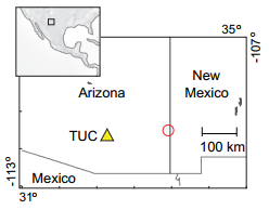
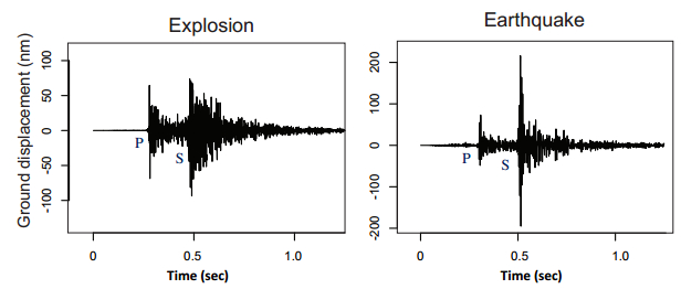
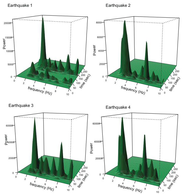
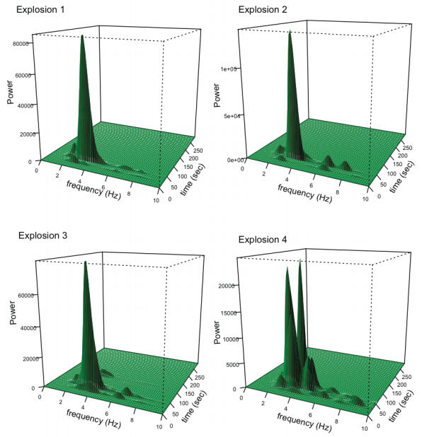
A sequence of intraplate earthquakes occurred in Arizona at the same location where mining explosions were carried out in previous years. The explosions and some of the earthquakes generated very similar seismic signals. In this study Dynamic Fourier Analysis is used for discriminating signals originating from natural earthquakes and mining explosions. Frequency analysis of seismograms recorded at regional distances shows that compared with the mining explosions the earthquake signals have larger amplitudes in the frequency interval ~ 6 to 8 Hz and significantly smaller amplitudes in the frequency interval ~ 2 to 4 Hz. This type of analysis permits identifying characteristics in the seismograms frequency yielding to detect potentially risky seismic events.
Citation: Maria C. Mariani, Hector Gonzalez-Huizar, Masum Md Al Bhuiyan, Osei K. Tweneboah. Using Dynamic Fourier Analysis to Discriminate Between Seismic Signals from Natural Earthquakes and Mining Explosions[J]. AIMS Geosciences, 2017, 3(3): 438-449. doi: 10.3934/geosci.2017.3.438
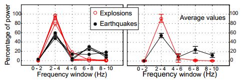
A sequence of intraplate earthquakes occurred in Arizona at the same location where mining explosions were carried out in previous years. The explosions and some of the earthquakes generated very similar seismic signals. In this study Dynamic Fourier Analysis is used for discriminating signals originating from natural earthquakes and mining explosions. Frequency analysis of seismograms recorded at regional distances shows that compared with the mining explosions the earthquake signals have larger amplitudes in the frequency interval ~ 6 to 8 Hz and significantly smaller amplitudes in the frequency interval ~ 2 to 4 Hz. This type of analysis permits identifying characteristics in the seismograms frequency yielding to detect potentially risky seismic events.

| [1] |
Kim WY, Aharonian V, Abbers G, et al. (1997) Discrimination of Earthquakes and Explosions in Southern Russia Using Regional High-Frequency Three-Component Data from the IRIS/JSP Caucasus Network. Bull Seismol Soc Am 87: 569-588. doi: 10.1785/BSSA0870030569

|
| [2] | Arrowsmith MD, Arrowsmith SJ, Stump B, et al. (2005) Discrimination of Small Events Using Regional Waveforms: Application to Seismic Events in the US and Russia. Proc 27th Seis Res Rev: Ground Based Nuclear Explos Monit Technol 498-508. |
| [3] | Xie J (2002) Source Scaling of Pn and Lg Spectra and Their Ratios from Explosions in Central Asia: Implications for the Identification of Small Seismic Events at Regional Distances. J Geophys Res 107: 2128. |
| [4] | Grunwald GK, Hyndman RJ, Tedesco LM (1996) A Unified View of Linear AR(1) Models. Unpublished paper. |
| [5] | Said SE, Dickey D (1984) Testing for Unit Roots in Autoregressive Moving-Average Models with Unknown Order. Biom 71: 599-607. |
| [6] | Zivot E, Wang J (2006) Modeling Financial Time Series with S-PLUS, Springer, 111-139. |
| [7] |
Beccar-Varela MP, Gonzalez-Huizar H, Mariani MC, et al. (2016) Use of Wavelets Techniques to Discriminate Between Explosions and Natural Earthquakes. Phys A: Stat Mech Appl 457: 42-51. doi: 10.1016/j.physa.2016.03.077
|
| [8] | Press WH, Teukolsky SA, Vetterling WT, et al. (1992) Numerical Recipes in C-The Art of Scientific Computing, 2 Eds. , Cambridge University Press, 537-545. |
| [9] | Shumway RH, Sto er DS (2010) Time Series Analysis and its Applications With R Examples, 3 Eds. , Springer, 230-235. |
| [10] | Cryer JD, Chan KS (2008) Time Series Analysis with its Applications in R, 2 Eds. , Springer, 351-367,322-328. |
| [11] | Gubbins D (2004) Time Series Analysis and Inverse Theory for Geophysicists. Camb Univ Press 47: 180-184. |
| [12] | Walter WR, Matzel E, Pasyanos ME, et al. (2007) Empirical Observations of Earthquake-Explosion Discrimination Using P/S Ratios and Implications for the Sources of Explosion S-Waves, Lawrence Livermore National Lab CA. 29th Research Review on Nuc Explo Monit Tech Denver CO United States. |
Figures(5) / Tables(4)

Maria C. Mariani, Hector Gonzalez-Huizar, Masum Md Al Bhuiyan, Osei K. Tweneboah. Using Dynamic Fourier Analysis to Discriminate Between Seismic Signals from Natural Earthquakes and Mining Explosions[J]. AIMS Geosciences, 2017, 3(3): 438-449. doi: 10.3934/geosci.2017.3.438


 DownLoad: