An Informer-based multi-scale model that fuses memory factors and wavelet denoising for tidal prediction

Peng Lu; Yuchen He; Wenhui Li; Yuze Chen; Ru Kong; Teng Wang; Peng Lu; Yuchen He; Wenhui Li; Yuze Chen; Ru Kong; Teng Wang

doi:10.3934/era.2025032

Electronic Research Archive

2025, Volume 33, Issue 2: 697-724. doi: 10.3934/era.2025032

Previous Article Next Article

Research article

An Informer-based multi-scale model that fuses memory factors and wavelet denoising for tidal prediction

1.
College of Information Technology, Shanghai Ocean University, Shanghai 201306, China
2.
Modern Educational Technology Center, Shanghai Maritime University, Shanghai 201306, China
3.
Shandong Provincial Institute of Land Space Data and Remote Sensing Technology, Shandong Ocean Bureau, Jinan 250002, China

Received: 22 September 2024 Revised: 18 November 2024 Accepted: 10 December 2024 Published: 11 February 2025

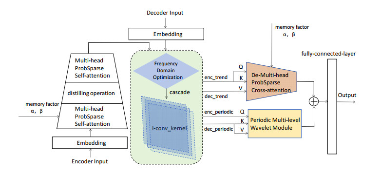
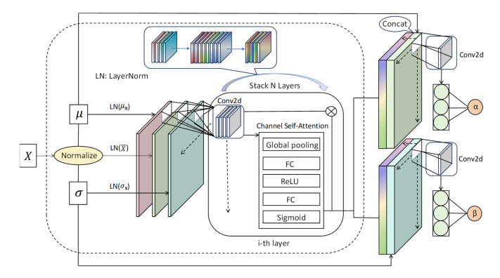
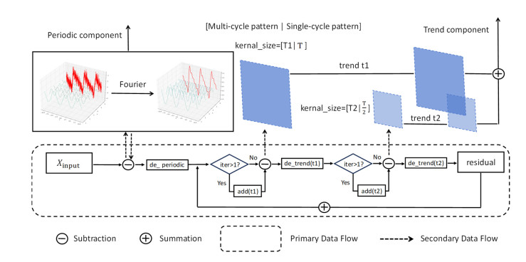
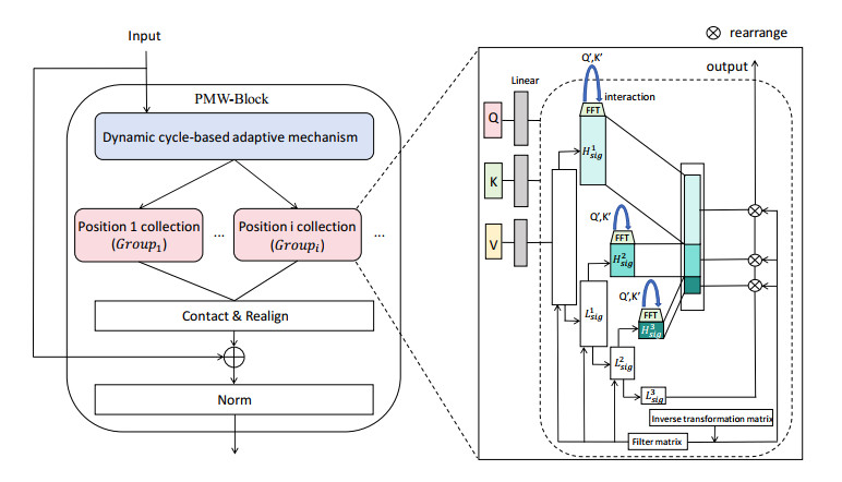
Tidal time series are affected by a combination of astronomical, geological, meteorological, and anthropogenic factors, revealing non-stationary and multi-period features. The statistical features of non-stationary data vary over time, making it challenging for typical time series forecasting models to capture their dynamism. To solve this challenge, we designed memory factors, leveraging the fusion of statistical data at the channel dimension to enhance the model's prediction capacity for non-stationary data. On the other hand, traditional approaches have limitations in trend and cycle decomposition, making it difficult to detect complicated multi-period patterns and accurately separate the components. We combined integrated frequency domain optimization and multi-level, multi-scale convolutional kernel technologies. By employing Fourier-based methods and iterative recursive decomposition strategies, we effectively separated periodic and trend components. Then, the periodic multi-level wavelet block was applied to extract the periodic interaction features, aiming to deeply mine the latent information of periodic components and enhance the model's long-term prediction capabilities. In this paper, we used the Informer model as the foundational framework for further research and development. In comparative experiments, our proposed model outperformed LSTM, Informer, and MICN by 61.4%, 51.7%, and 23.8%, respectively. In multi-time-span prediction, the model's error remained stable as the prediction span increased from 48 to 96 steps (from 0.059 to 0.067). Under multi-site conditions, the model achieved varying degrees of improvement over the baseline in three key evaluation metrics, with average increases of 35.2%, 35.6%, and 61.2%, respectively. In this study, we focused on the extraction of short-period features from tidal data, providing an innovative and reliable solution for tidal height prediction. The results are significant for tidal assessments and protective engineering construction.
- tidal prediction,
- time series,
- Informer,
- memory factor,
- multi-scale convolution,
- multi-level wavelet
Citation: Peng Lu, Yuchen He, Wenhui Li, Yuze Chen, Ru Kong, Teng Wang. An Informer-based multi-scale model that fuses memory factors and wavelet denoising for tidal prediction[J]. Electronic Research Archive, 2025, 33(2): 697-724. doi: 10.3934/era.2025032

Related Papers:

Abstract

Tidal time series are affected by a combination of astronomical, geological, meteorological, and anthropogenic factors, revealing non-stationary and multi-period features. The statistical features of non-stationary data vary over time, making it challenging for typical time series forecasting models to capture their dynamism. To solve this challenge, we designed memory factors, leveraging the fusion of statistical data at the channel dimension to enhance the model's prediction capacity for non-stationary data. On the other hand, traditional approaches have limitations in trend and cycle decomposition, making it difficult to detect complicated multi-period patterns and accurately separate the components. We combined integrated frequency domain optimization and multi-level, multi-scale convolutional kernel technologies. By employing Fourier-based methods and iterative recursive decomposition strategies, we effectively separated periodic and trend components. Then, the periodic multi-level wavelet block was applied to extract the periodic interaction features, aiming to deeply mine the latent information of periodic components and enhance the model's long-term prediction capabilities. In this paper, we used the Informer model as the foundational framework for further research and development. In comparative experiments, our proposed model outperformed LSTM, Informer, and MICN by 61.4%, 51.7%, and 23.8%, respectively. In multi-time-span prediction, the model's error remained stable as the prediction span increased from 48 to 96 steps (from 0.059 to 0.067). Under multi-site conditions, the model achieved varying degrees of improvement over the baseline in three key evaluation metrics, with average increases of 35.2%, 35.6%, and 61.2%, respectively. In this study, we focused on the extraction of short-period features from tidal data, providing an innovative and reliable solution for tidal height prediction. The results are significant for tidal assessments and protective engineering construction.

References

[1]	T. Bongarts Lebbe, H. Rey-Valette, É. Chaumillon, G. Camus, R. Almar, A. Cazenave, et al., Designing coastal adaptation strategies to tackle sea level rise, Front. Mar. Sci., 8 (2021), 740602. https://doi.org/10.3389/fmars.2021.740602 doi: 10.3389/fmars.2021.740602
[2]	G. Griggs, B. G. Reguero, Coastal adaptation to climate change and sea-level rise, Water, 13 (2021), 2151. https://doi.org/10.3390/w13162151 doi: 10.3390/w13162151
[3]	A. T. Doodson, The analysis and predictions of tides in shallow water, Int. Hydrogr. Rev., 33 (1958), 85–126.
[4]	R. E. Kalman, A new approach to linear filtering and prediction problems, J. Basic Eng., 82 (1960), 35–45. https://doi.org/10.1115/1.3662552 doi: 10.1115/1.3662552
[5]	G. Evensen, Sequential data assimilation with a nonlinear quasi-geostrophic model using Monte Carlo methods to forecast error statistics, J. Geophys. Res., 99 (1994), 10143–10162. https://doi.org/10.1029/94JC00572 doi: 10.1029/94JC00572
[6]	Y. Yang, Y. Gao, Z. Wang, X. Li, H. Zhou, J. Wu, Multiscale-integrated deep learning approaches for short-term load forecasting, Int. J. Mach. Learn. Cybern., 15 (2024), 6061–6076. https://doi.org/10.1007/s13042-024-02302-4 doi: 10.1007/s13042-024-02302-4
[7]	S. Zhang, Z. Zhao, J. Wu, Y. Jin, D. S. Jeng, S. Li, et al., Solving the temporal lags in local significant wave height prediction with a new VMD-LSTM model, Ocean Eng., 313 (2024), 119385. https://doi.org/10.1016/j.oceaneng.2024.119385 doi: 10.1016/j.oceaneng.2024.119385
[8]	J. C. Yin, A. N. Perakis, N. Wang, An ensemble real-time tidal level prediction mechanism using multiresolution wavelet decomposition method, IEEE Trans. Geosci. Remote Sensing, 56 (2018), 4856–4865. https://doi.org/10.1109/TGRS.2018.2841204 doi: 10.1109/TGRS.2018.2841204
[9]	T. L. Lee, Back-propagation neural network for long-term tidal predictions, Ocean Eng., 31 (2004), 225–238. https://doi.org/10.1016/S0029-8018(03)00115-X doi: 10.1016/S0029-8018(03)00115-X
[10]	N. Portillo Juan, V. Negro Valdecantos, Review of the application of artificial neural networks in ocean engineering, Ocean Eng., 259 (2022), 111947. https://doi.org/10.1016/j.oceaneng.2022.111947 doi: 10.1016/j.oceaneng.2022.111947
[11]	C. L. Giles, G. M. Kuhn, R. J. Williams, Dynamic recurrent neural networks: Theory and applications, IEEE Trans. Neural Netw., 5 (1994), 153–156. https://doi.org/10.1109/TNN.1994.8753425 doi: 10.1109/TNN.1994.8753425
[12]	S. Fan, N. Xiao, S. Dong, A novel model to predict significant wave height based on long short-term memory network, Ocean Eng., 205 (2020), 107298. https://doi.org/10.1016/j.oceaneng.2020.107298 doi: 10.1016/j.oceaneng.2020.107298
[13]	L. H. Bai, H. Xu, Accurate estimation of tidal level using bidirectional long short-term memory recurrent neural network, Ocean Eng., 235 (2021), 108765. https://doi.org/10.1016/j.oceaneng.2021.108765 doi: 10.1016/j.oceaneng.2021.108765
[14]	Q. R. Luo, H. Xu, L. H. Bai, Prediction of significant wave height in hurricane area of the Atlantic Ocean using the Bi-LSTM with attention model, Ocean Eng., 266 (2022), 112747. https://doi.org/10.1016/j.oceaneng.2022.112747 doi: 10.1016/j.oceaneng.2022.112747
[15]	J. Oh, K. D. Suh, Real-time forecasting of wave heights using EOF-wavelet-neural network hybrid model, Ocean Eng., 150 (2018), 48–59. https://doi.org/10.1016/j.oceaneng.2017.12.044 doi: 10.1016/j.oceaneng.2017.12.044
[16]	H. H. H. Aly, Intelligent optimised deep learning hybrid models of neuro wavelet, Fourier series and recurrent Kalman filter for tidal currents constitutions forecasting, Ocean Eng., 218 (2020), 108254. https://doi.org/10.1016/j.oceaneng.2020.108254 doi: 10.1016/j.oceaneng.2020.108254
[17]	A. Vaswani, N. Shazeer, N. Parmar, J. Uszkoreit, L. Jones, A. N. Gomez, et al., Attention is all you need, in Advances in Neural Information Processing Systems, 30 (2017), 5998–6008. https://doi.org/10.48550/arXiv.1706.03762
[18]	S. Wang, Z. Huang, B. Zhang, X. Heng, Y. Jiang, X. Sun, Plot-aware Transformer for recommender systems, Electron. Res. Arch., 31 (2023), 3169–3186. https://doi.org/10.3934/era.2023160 doi: 10.3934/era.2023160
[19]	Y. Li, X. Wang, Y. Guo, CNN-Trans-SPP: A small Transformer with CNN for stock price prediction, Electron. Res. Arch., 32 (2024), 6717–6732. https://doi.org/10.3934/era.2024314 doi: 10.3934/era.2024314
[20]	J. Wan, N. Xia, Y. Yin, X. Pan, J. Hu, J. Yi, TCDformer: A transformer framework for non-stationary time series forecasting based on trend and change-point detection, Neural Netw., 173 (2024), 106196. https://doi.org/10.1016/j.neunet.2024.106196 doi: 10.1016/j.neunet.2024.106196
[21]	H. Zhou, S. Zhang, J. Peng, S. Zhang, J. Li, H. Xiong, et al., Informer: Beyond efficient transformer for long sequence time-series forecasting, in Proceedings of the AAAI Conference on Artificial Intelligence, 35 (2021), 11106–11115. https://doi.org/10.48550/arXiv.2012.07436
[22]	H. Wu, J. Xu, J. Wang, M. Long, Autoformer: Decomposition transformers with auto-correlation for long-term series forecasting, Adv. Neural Inf. Process. Syst., 34 (2021), 22419–22430. https://doi.org/10.48550/arXiv.2106.13008 doi: 10.48550/arXiv.2106.13008
[23]	T. Zhou, Z. Ma, Q. Wen, X. Wang, L. Sun, R. Jin, FEDformer: Frequency enhanced decomposed transformer for long-term series forecasting, J. Int. Law Policy, 3 (2022), 321–322. https://doi.org/10.48550/arXiv.2201.12740 doi: 10.48550/arXiv.2201.12740
[24]	Y. Nie, N. H. Nguyen, P. Sinthong, J. Kalagnanam, A time series is worth 64 words: Long-term forecasting with transformers, in International Conference on Learning Representations, (2022). https://doi.org/10.48550/arXiv.2211.14730
[25]	Y. Liu, H. Wu, J. Wang, M. Long, Non-stationary transformers: exploring the stationarity in time series forecasting, preprint, arXiv: 2205.14415. https://doi.org/10.48550/arXiv.2205.14415
[26]	Y. Liu, T. Hu, H. Zhang, H. Wu, S. Wang, L. Ma, M. Long, iTransformer: inverted transformers are effective for time series forecasting, J. Int. Law Policy, 3 (2023), 321–322. https://doi.org/10.48550/arXiv.2310.06625 doi: 10.48550/arXiv.2310.06625
[27]	Y. H. H. Tsai, S. Bai, M. Yamada, L. P. Morency, R. Salakhutdinov, Transformer dissection: A unified understanding of transformer's attention via the lens of kernel, preprint, arXiv: 1908.11775. https://doi.org/10.48550/arXiv.1908.11775
[28]	S. G. Mallat, A theory for multiresolution signal decomposition: the wavelet representation, IEEE Trans. Pattern Anal. Mach. Intell., 11 (1989), 674–693. https://doi.org/10.1109/34.192463 doi: 10.1109/34.192463
[29]	S. G. Venkatesh, S. K. Ayyaswamy, S. Raja Balachandar, The Legendre wavelet method for solving initial value problems of Bratu-type, Comput. Math. Appl., 63 (2012), 1287–1295. https://doi.org/10.1016/j.camwa.2011.12.069 doi: 10.1016/j.camwa.2011.12.069
[30]	A. A. Abdulrahman, F. S. Tahir, Face recognition using enhancement discrete wavelet transform based on MATLAB, Int. J. Eng. Comput. Sci., 23 (2021), 1128–1136. https://doi.org/10.11591/ijeecs.v23.i2.pp1128-1136 doi: 10.11591/ijeecs.v23.i2.pp1128-1136
[31]	N. Zheng, H. Chai, Y. Ma, L. Chen, P. Chen, Hourly sea level height forecast based on GNSS-IR by using ARIMA model, Remote Sens., 43 (2022), 3387–3411. https://doi.org/10.1080/01431161.2022.2091965 doi: 10.1080/01431161.2022.2091965
[32]	D. Lee, S. Lee, J. Lee, Standardization in building an ANN-based mooring line top tension prediction system, Int. J. Nav. Archit. Ocean Eng., 14 (2022), 100421. https://doi.org/10.1016/j.ijnaoe.2021.11.004 doi: 10.1016/j.ijnaoe.2021.11.004
[33]	J. Hu, L. Shen, G. Sun, Squeeze-and-excitation networks, in Proceedings of the 2018 IEEE/CVF Conference on Computer Vision and Pattern Recognition, (2018), 7132–7141. https://doi.org/10.1109/CVPR.2018.00745
[34]	H. Han, Z. Liu, M. Barrios, J. Li, Z. Zeng, N. Sarhan, et al., Time series forecasting model for non-stationary series pattern extraction using deep learning and GARCH modelling, J. Cloud Comput., 13 (2024), 2. https://doi.org/10.1186/s13677-023-00576-7 doi: 10.1186/s13677-023-00576-7
[35]	I. Yanovitzky, A. VanLear, Time series analysis: Traditional and contemporary approaches, in The SAGE Sourcebook of Advanced Data Analysis Methods for Communication Research (eds. A. F. Hayes, M. D. Slater, L. B. Snyder), Sage Publications, (2008), 89–124. https://doi.org/10.4135/9781452272054.n4
[36]	R. B. Cleveland, W. S. Cleveland, J. E. McRae, I. Terpenning, STL: A seasonal-trend decomposition procedure based on loess, J. Off. Stat., 6 (1990), 3–73.
[37]	C. Nontapa, C. Kesamoon, N. Kaewhawong, P. Intrapaiboon, A new time series forecasting using decomposition method with SARIMAX model, in Neural Information Processing, Communications in Computer and Information Science, 1333 (2020), 743–751. https://doi.org/10.1007/978-3-030-63823-8_84
[38]	T. Kim, B. R. King, Time series prediction using deep echo state networks, Neural Comput. Appl., 32 (2020), 17769–17787. https://doi.org/10.1007/s00521-020-04948-x doi: 10.1007/s00521-020-04948-x
[39]	H. Wu, T. Hu, Y. Liu, H. Zhou, J. Wang, M. Long, TimesNet: Temporal 2D-variation modeling for general time series analysis, in International Conference on Learning Representations, (2022). https://doi.org/10.48550/arXiv.2210.02186
[40]	A. R. Abdullah, N. M. Saad, A. Zuri, Power quality monitoring system utilizing periodogram and spectrogram analysis techniques, in Asean Virtual Instrumentation Applications Contest, (2007). https://doi.org/10.13140/2.1.3109.1841
[41]	C. Samson, V. U. K. Sastry, A novel image encryption supported by compression using multilevel wavelet transform, Int. J. Adv. Comput. Sci. Appl., 3 (2012). https://doi.org/10.14569/IJACSA.2012.030926
[42]	S. Liu, H. Yu, C. Liao, J. Li, W. Lin, A. X. Liu, et al., Pyraformer: low-complexity pyramidal attention for long-range time series modelling and forecasting, in Proceedings of the 10th International Conference on Learning Representations, 2022. Available from: https://openreview.net/forum?id = 0EXmFzUn5I.
[43]	H. Wang, J. Peng, F. Huang, J. Wang, J. Chen, Y. Xiao, MICN: Multi-scale local and global context modelling for long-term series forecasting, in International Conference on Learning Representations, 2023. Available from: https://openreview.net/forum?id = zt53IDUR1U.
[44]	M. Liu, A. Zeng, M. Chen, Z. Xu, Q. Lai, L. Ma, et al., SCINet: time series modelling and forecasting with sample convolution and interaction, in Advances in Neural Information Processing Systems, 35 (2022), 5816–5828. https://doi.org/10.48550/arXiv.2106.09305
[45]	A. Zeng, M. Chen, L. Zhang, Q. Xu, Are transformers effective for time series forecasting?, in Proceedings of the AAAI Conference on Artificial Intelligence, 37 (2023), 11121–11128. https://doi.org/10.48550/arXiv.2205.13504

Reader Comments

Your name:*

Email:*
© 2025 the Author(s), licensee AIMS Press. This is an open access article distributed under the terms of the Creative Commons Attribution License (http://creativecommons.org/licenses/by/4.0)