Modelling and analysis of a delayed viral infection model with follicular dendritic cell

Yan Geng; Jinhu Xu; Yan Geng; Jinhu Xu

doi:10.3934/era.2024236

Electronic Research Archive

2024, Volume 32, Issue 8: 5127-5138. doi: 10.3934/era.2024236

Previous Article Next Article

Research article

Modelling and analysis of a delayed viral infection model with follicular dendritic cell

Yan Geng ¹,
Jinhu Xu ^{2
,
,}

1.
School of Science, Xi'an Polytechnic University, Xi'an 710048, China
2.
School of Sciences, Xi'an University of Technology, Xi'an 710048, China

Received: 14 July 2024 Revised: 11 August 2024 Accepted: 19 August 2024 Published: 29 August 2024

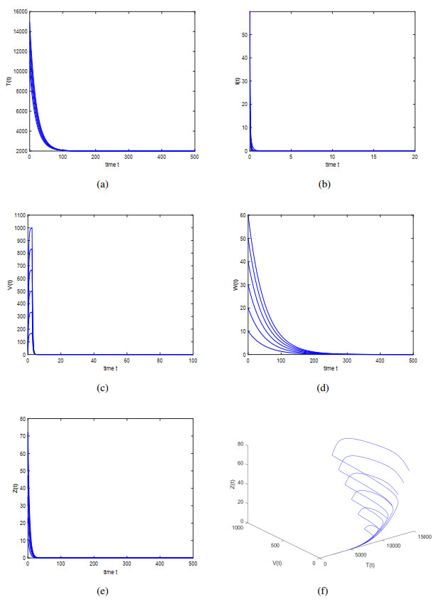
In this paper, we propose a new viral infection model by incorporating a new compartment for follicular dendritic cell (FDC), nonlinear incidence, CTL immune response, and two intracellular delays. The main purpose of the paper is to make an improvement and supplement to the global dynamics of the model proposed by Callaway and Perelson (2002), in which global stability has not been studied. The global stabilities of equilibria are established by constructing corresponding Lyapunov functionals in terms of two threshold parameters, $ \mathfrak{R}_0 $ and $ \mathfrak{R}_1 $. The obtained results imply that both nonlinear incidence and intracellular time delays have no impact on the stability of the model.
- follicular dendritic cell,
- intracellular time delays,
- nonlinear incidence,
- global stability,
- Lyapunov functionals
Citation: Yan Geng, Jinhu Xu. Modelling and analysis of a delayed viral infection model with follicular dendritic cell[J]. Electronic Research Archive, 2024, 32(8): 5127-5138. doi: 10.3934/era.2024236

Related Papers:

Abstract

In this paper, we propose a new viral infection model by incorporating a new compartment for follicular dendritic cell (FDC), nonlinear incidence, CTL immune response, and two intracellular delays. The main purpose of the paper is to make an improvement and supplement to the global dynamics of the model proposed by Callaway and Perelson (2002), in which global stability has not been studied. The global stabilities of equilibria are established by constructing corresponding Lyapunov functionals in terms of two threshold parameters, $ \mathfrak{R}_0 $ and $ \mathfrak{R}_1 $. The obtained results imply that both nonlinear incidence and intracellular time delays have no impact on the stability of the model.

References

[1]	A. S. Perelson, D. E. Kirschner, R. D. Boer, Dynamics of HIV infection of CD4+ T cells, Math. Biosci., 114 (1993), 81–125. https://doi.org/10.1016/0025-5564(93)90043-A doi: 10.1016/0025-5564(93)90043-A
[2]	A. S. Perelson, P. W. Nelson, Mathematical analysis of HIV-1 dynamics in vivo, SIAM Rev., 41 (1999), 3–44. https://doi.org/10.1137/S0036144598335107 doi: 10.1137/S0036144598335107
[3]	A. S. Perelson, A. U. Neumann, M. Markowitz, J. M. Leonard, D. D. Ho, HIV-1 dynamics in vivo: virion clearance rate, infected cell life-span, and viral generation time, Science, 271 (1996), 1582–1586. https://doi.org/10.1126/science.271.5255.1582 doi: 10.1126/science.271.5255.1582
[4]	S. Bonhoeffer, R. M. May, G. M. Shaw, M. A. Nowak, Virus dynamics and drug therapy, Proc. Natl. Acad. Sci., 94 (1997), 6971–6976. https://doi.org/10.1073/pnas.94.13.6971 doi: 10.1073/pnas.94.13.6971
[5]	M. A. Nowak, C. R. M. Bangham, Population dynamics of immune responses to persistent viruses, Science, 272 (1996), 74–79. https://doi.org/10.1126/science.272.5258.74 doi: 10.1126/science.272.5258.74
[6]	X. Wang, Y. Tao, X. Song, Global stability of a virus dynamics model with Beddington-DeAngelis incidence tate and CTL immune response, Nonlinear Dynam., 66 (2011), 825–830. https://doi.org/10.1007/s11071-011-9954-0 doi: 10.1007/s11071-011-9954-0
[7]	H. Shu, L. Wang, J. Watmough, Global stability of a nonlinear viral infection model with infinitely distributed intracellular delays and CTL immune responses, SIAM J. Appl. Math., 73 (2013), 1280–1302. https://doi.org/10.1137/120896463 doi: 10.1137/120896463
[8]	S. S. Chen, C. Y. Cheng, Y. Takeuchi, Stability analysis in delayed within-host viral dynamics with both viral and cellular infections, J. Math. Anal. Appl., 442 (2016), 642–672. https://doi.org/10.1016/j.jmaa.2016.05.003 doi: 10.1016/j.jmaa.2016.05.003
[9]	W. S. Hlavacek, C. Wofsy, A. S. Perelson, Dissociation of HIV-1 from follicular dendritic cells during HAART: mathematical analysis, Proc. Nat. Acad. Sci., 96 (1999), 14681–14686. https://doi.org/10.1073/pnas.96.26.14681 doi: 10.1073/pnas.96.26.14681
[10]	W. S. Hlavacek, N. I. Stilianakis, D. W. Notermans, S. A. Danner, A. S. Perelson, Influence of follicular dendritic cells on decay of HIV during antiretroviral therapy, Proc. Nat. Acad. Sci., 97 (2000), 10966–10971. https://doi.org/10.1073/pnas.190065897 doi: 10.1073/pnas.190065897
[11]	D. S. Callaway, A. S. Perelson, HIV-1 infection and low steady state viral loads, Bull. Math. Biol., 64 (2002), 29–64. https://doi.org/10.1006/bulm.2001.0266 doi: 10.1006/bulm.2001.0266
[12]	T. C. Thacker, X. Zhou, J. D. Estes, Y. Jiang, B. F. Keele, T. S. Elton, et al., Follicular dendritic cells and human immunodeficiency virus type 1 transcription in CD4+ T cells, J. Virol., 83 (2009), 150–158. https://doi.org/10.1128/jvi.01652-08 doi: 10.1128/jvi.01652-08
[13]	E. L. Shikh, E. M. Mohey, Costantino Pitzalis. Follicular dendritic cells in health and disease, Front. Immunol., 3 (2012), 31755. https://doi.org/10.3389/fimmu.2012.00292 doi: 10.3389/fimmu.2012.00292
[14]	J. Zhang, A. S. Perelson, Contribution of follicular dendritic cells to persistent HIV viremia, J. Virol., 87 (2013), 7893–7901. https://doi.org/10.1128/jvi.00556-13 doi: 10.1128/jvi.00556-13
[15]	F. Sabri, A. Prados, R. Mu$\tilde{n}$oz-Fern$\acute{a}$ndez, R. Lantto, P. Fernandez-Rubio, A. Nasi, et al., Impaired B cells survival upon production of inflammatory cytokines by HIV-1 exposed follicular dendritic cells, Retrovirology, 13 (2016). https://doi.org/10.1186/s12977-016-0295-4 doi: 10.1186/s12977-016-0295-4
[16]	C. V. Fletcher, K. Staskus, S. W. Wietgrefe, et al., Persistent HIV-1 replication is associated with lower antiretroviral drug concentrations in lymphatic tissues, Proc. Natl. Acad. Sci., 111 (2014), 2307–2312. https://doi.org/10.1073/pnas.1318249111 doi: 10.1073/pnas.1318249111
[17]	M. T. Ollerton, E. A. Berger, E. Connick, G. F. Burton, HIV-1-specific chimeric antigen receptor T cells fail to recognize and eliminate the follicular dendritic cell HIV reservoir in vitro, J. Virol., 94 (2020). https://doi.org/10.1128/jvi.00190-20 doi: 10.1128/jvi.00190-20
[18]	M. S. Ciupe, B. L. Bivort, D. M. Bortz, P. W. Nelson, Estimating kinetic parameters from HIV primary infection data through the eyes of three different mathematical models, Math. Biosci., 200 (2006). https://doi.org/10.1016/j.mbs.2005.12.006 doi: 10.1016/j.mbs.2005.12.006
[19]	X. Yang, L. Chen, J Chen, Permanence and positive periodic solution for the single-species nonautonomous delay diffusive models, Comput. Math. Appl., 32 (1996), 109–116. https://doi.org/10.1016/0898-1221(96)00129-0 doi: 10.1016/0898-1221(96)00129-0
[20]	A. Korobeinikov, Global properties of basic virus dynamics models, Bull. Math. Biol., 66 (2004), 879–883. https://doi.org/10.1016/j.bulm.2004.02.001 doi: 10.1016/j.bulm.2004.02.001
[21]	C. C. McCluskey, Complete global stablity for an SIR epidemic model with delay-distributed or discrete, Nonlinear Anal. Real World Appl., 11 (2010), 55–59. https://doi.org/10.1016/j.nonrwa.2008.10.014 doi: 10.1016/j.nonrwa.2008.10.014
[22]	K. Hattaf, N. Yousfi, Global stability for reaction-diffusion equations in biology, Comput. Math. Appl., 66 (2013), 1488–1497. https://doi.org/10.1016/j.camwa.2013.08.023 doi: 10.1016/j.camwa.2013.08.023
[23]	K. Hattaf, N. Yousfi, A generalized HBV model with diffusion and two delays, Comput. Math. Appl., 69 (2015), 31–40. https://doi.org/10.1016/j.camwa.2014.11.010 doi: 10.1016/j.camwa.2014.11.010
[24]	J. K. Hale, S. M. V. Lunel, Introduction to Functional Differential Equations, Springer-Verlag, New York, 1993. https://doi.org/10.1007/978-1-4612-4342-7
[25]	S. Gummuluru, C. M. Kinsey, M. Emerman, An in vitro rapid-turnover assay for human immunodeficiency virus type 1 replication selects for cell-to-cell spread of virus, J. Virol., 74 (2000), 10882–10891. https://doi.org/10.1128/JVI.74.23.10882-10891.2000 doi: 10.1128/JVI.74.23.10882-10891.2000
[26]	C. R. M. Bangham, The immune control and cell-to-cell spread of human T-lymphotropic virus type 1, J. Gen. Virol., 84 (2003), 3177–3189. https://doi.org/10.1099/vir.0.19334-0 doi: 10.1099/vir.0.19334-0
[27]	A. Sigal, J. T. Kim, A. B. Balazs, E. Dekel, A. Mayo, R. Milo, et al., Cell-to-cell spread of HIV permits ongoing replication despite antiretroviral therapy, Nature, 477 (2011), 95–98. https://doi.org/10.1038/nature10347 doi: 10.1038/nature10347

Reader Comments

Your name:*

Email:*
© 2024 the Author(s), licensee AIMS Press. This is an open access article distributed under the terms of the Creative Commons Attribution License (http://creativecommons.org/licenses/by/4.0)