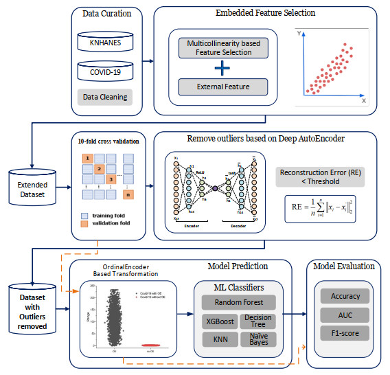
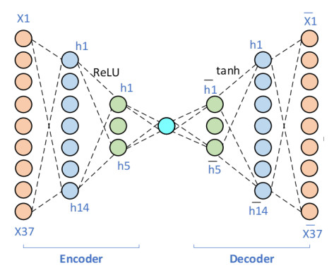
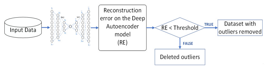
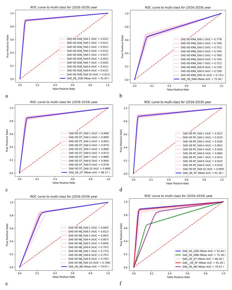
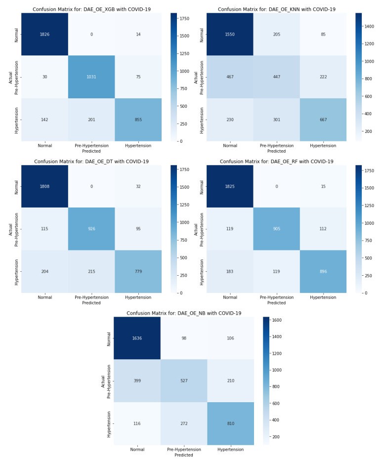
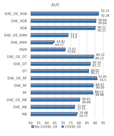
The incidence of hypertension has increased dramatically in both elderly and young populations. The incidence of hypertension also increased with the outbreak of the COVID-19 pandemic. To enhance hypertension detection accuracy, we proposed a multivariate outlier removal method based on the deep autoencoder (DAE) technique. The method was applied to the Korean National Health and Nutrition Examination Survey (KNHANES) database. Several studies have identified various risk factors for chronic hypertension. Chronic diseases are often multifactorial rather than isolated and have been associated with COVID-19. Therefore, it is necessary to study disease detection by considering complex factors. This study was divided into two main parts. The first module, data preprocessing, integrated external features for COVID-19 patients merged by region, age, and gender for the KHNANE-2020 and Kaggle datasets. We then performed multicollinearity (MC)-based feature selection for the KNHANES and integrated datasets. Notably, our MC analysis revealed that the "COVID-19 statement" feature, with a variance inflation factor (VIF) of 1.023 and a p-value < 0.01, is significant in predicting hypertension, underscoring the interrelation between COVID-19 and hypertension risk. The next module used a predictive analysis step to detect and predict hypertension based on an ordinal encoder (OE) transformation and multivariate outlier removal using a DAE from the KNHANES data. We compared each classification model's accuracy, F1 score, and area under the curve (AUC). The experimental results showed that the proposed XGBoost model achieved the best results, with an accuracy rate of 87.78% (86.49%–88.1%, 95% CI), an F1 score of 89.95%, and an AUC of 92.28% for the COVID-19 cases, and an accuracy rate of 87.72% (85.86%–89.69%, 95% CI), an F1 score of 89.94%, and an AUC of 92.23% for the non-COVID-19 cases with the DAE_OE model. We improved the prediction performance of the classifiers used in all experiments by developing a high-quality training dataset implementing the DAE and OE in our method. Moreover, we experimentally demonstrated how the steps of the proposed method improved performance. Our approach has potential applications beyond hypertension detection, including other diseases such as stroke and cardiovascular disease.
Citation: Khongorzul Dashdondov, Mi-Hye Kim, Mi-Hwa Song. Deep autoencoders and multivariate analysis for enhanced hypertension detection during the COVID-19 era[J]. Electronic Research Archive, 2024, 32(5): 3202-3229. doi: 10.3934/era.2024147
The incidence of hypertension has increased dramatically in both elderly and young populations. The incidence of hypertension also increased with the outbreak of the COVID-19 pandemic. To enhance hypertension detection accuracy, we proposed a multivariate outlier removal method based on the deep autoencoder (DAE) technique. The method was applied to the Korean National Health and Nutrition Examination Survey (KNHANES) database. Several studies have identified various risk factors for chronic hypertension. Chronic diseases are often multifactorial rather than isolated and have been associated with COVID-19. Therefore, it is necessary to study disease detection by considering complex factors. This study was divided into two main parts. The first module, data preprocessing, integrated external features for COVID-19 patients merged by region, age, and gender for the KHNANE-2020 and Kaggle datasets. We then performed multicollinearity (MC)-based feature selection for the KNHANES and integrated datasets. Notably, our MC analysis revealed that the "COVID-19 statement" feature, with a variance inflation factor (VIF) of 1.023 and a p-value < 0.01, is significant in predicting hypertension, underscoring the interrelation between COVID-19 and hypertension risk. The next module used a predictive analysis step to detect and predict hypertension based on an ordinal encoder (OE) transformation and multivariate outlier removal using a DAE from the KNHANES data. We compared each classification model's accuracy, F1 score, and area under the curve (AUC). The experimental results showed that the proposed XGBoost model achieved the best results, with an accuracy rate of 87.78% (86.49%–88.1%, 95% CI), an F1 score of 89.95%, and an AUC of 92.28% for the COVID-19 cases, and an accuracy rate of 87.72% (85.86%–89.69%, 95% CI), an F1 score of 89.94%, and an AUC of 92.23% for the non-COVID-19 cases with the DAE_OE model. We improved the prediction performance of the classifiers used in all experiments by developing a high-quality training dataset implementing the DAE and OE in our method. Moreover, we experimentally demonstrated how the steps of the proposed method improved performance. Our approach has potential applications beyond hypertension detection, including other diseases such as stroke and cardiovascular disease.

| [1] | Korea Centers for Disease Control & Prevention. http://knhanes.cdc.go.kr. Accessed: February 4, 2014. |
| [2] |
C. Wang, P. W. Horby, F. G. Hayden, G. F. Gao, A novel coronavirus outbreak of global health concern, Lancet, 395 (2020), 470–473. https://doi.org/10.1016/S0140-6736(20)30185-9 doi: 10.1016/S0140-6736(20)30185-9

|
| [3] | World Health Organization, https://www.who.int/health-topics/hypertension/#tab = tab_1 |
| [4] | D. Khongorzul, M. H. Kim, Mahalanobis distance based multivariate outlier detection to improve performance of hypertension prediction, Neural Process. Lett., (2021), 1–13. |
| [5] |
B. Liao, X. Jia, T. Zhang, R. Sun, DHDIP: An interpretable model for hypertension and hyperlipidemia prediction based on EMR data, Comput. Methods Programs Biomed., 226 (2022), 107088. https://doi.org/10.1016/j.cmpb.2022.107088 doi: 10.1016/j.cmpb.2022.107088
|
| [6] |
I. Baik, Region-specific COVID-19 risk scores and nutritional status of a high-risk population based on individual vulnerability assessment in the national survey data, Clin. Nutr., 41 (2022), 3100–3105. https://doi.org/10.1016/j.clnu.2021.02.019 doi: 10.1016/j.clnu.2021.02.019
|
| [7] |
J. Kim, K. K. Byon, Leisure activities, happiness, life satisfaction, and health perception of older Korean adults. Int. J. Ment Health Promot., 23 (2021), 155–166. https://doi.org/10.32604/IJMHP.2021.015232 doi: 10.32604/IJMHP.2021.015232
|
| [8] |
J. Y. Kwon, S. W Song, Changes in the prevalence of metabolic syndrome in Korean adults after the COVID-19 outbreak, Epidemiol. Health, 5 (2022), e2022101. https://doi.org/10.4178/epih.e2022101 doi: 10.4178/epih.e2022101
|
| [9] |
K. Song, S. Y. Jung, J. Yang, H. S. Lee, H. S. Kim, H. W. Chae, Change in prevalence of hypertension among Korean children and adolescents during the COVID-19 outbreak: A population-based study, Children, 10 (2023), 159. https://doi.org/10.3390/children10010159 doi: 10.3390/children10010159
|
| [10] |
H. Jeong, H. W. Yim, S. Y. Lee, Impact of the COVID-19 pandemic on gender differences in depression based on national representative data, J. Korean Med. Sci., 38 (2023), 6. https://doi.org/10.3346/jkms.2023.38.e36 doi: 10.3346/jkms.2023.38.e36
|
| [11] |
H. D. Nguyen, H. Oh, M. S. Kim, The association between curry-rice consumption and hypertension, type 2 diabetes, and depression: The findings from KNHANES 2012–2016, Diabetes Metab. Syndr., 16 (2022), 102378. https://doi.org/10.1016/j.dsx.2021.102378 doi: 10.1016/j.dsx.2021.102378
|
| [12] |
A. Sumathi, S. Meganathan, B. V. Ravisankar, An intelligent gestational diabetes diagnosis model using deep stacked autoencoder, Comput. Mater. Contin., 69 (2021), 3109–3126. https://doi.org/10.32604/cmc.2021.017612 doi: 10.32604/cmc.2021.017612
|
| [13] |
Y. D. Zhang, M. A. Khan, Z. Zhu, S. H. Wang, Pseudo zernike moment and deep stacked sparse autoencoder for COVID-19 diagnosis, Comput. Mater. Contin., 69 (2021), 3145–3162. https://doi.org/10.32604/cmc.2021.018040 doi: 10.32604/cmc.2021.018040
|
| [14] |
H. Dhahri, B. Rabhi, S. Chelbi, O. Almutiry, A. Mahmood, A. M. Alimi, Automatic detection of COVID-19 using a stacked senoising convolutional autoencoder, Comput. Mater. Contin., 69 (2021), 3259–3274. https://doi.org/10.32604/cmc.2021.018449 doi: 10.32604/cmc.2021.018449
|
| [15] |
M. A. Hamza, S. B. Hassine, I. Abunadi, F. N. Al-Wesabi, H. Alsolai, A. M. Hilal, et al., Feature selection with optimal stacked sparse autoencoder for data mining, Comput. Mater. Contin., 72 (2022), 2581–2596. https://doi.org/10.32604/cmc.2022.024764 doi: 10.32604/cmc.2022.024764
|
| [16] |
M. Fang, Y. Chen, R. Xue, H. Wang, N. Chakraborty, T. Su, et al., A hybrid machine learning approach for hypertension risk prediction, Neural Comput. Appl., 35 (2023), 14487–14497. https://doi.org/10.1007/s00521-021-06060-0 doi: 10.1007/s00521-021-06060-0
|
| [17] |
H. Kanegae, K. Suzuki, K. Fukatani, T. Ito, N. Harada, K. Kario, Highly precise risk prediction model for new-onset hypertension using artificial intelligence techniques. J. Clin. Hyper., 22 (2020), 445–450. https://doi.org/10.1111/jch.13759 doi: 10.1111/jch.13759
|
| [18] |
L. A. AlKaabi, L. S. Ahmed, M. F. Al Attiyah, M. E. Abdel-Rahman, Predicting hypertension using machine learning: Findings from Qatar biobank study, Plos One, 15 (2020), e0240370. https://doi.org/10.1371/journal.pone.0240370 doi: 10.1371/journal.pone.0240370
|
| [19] |
F. López-Martínez, E. R. Núñez-Valdez, R. G. Crespo, V. García-Díaz, An artificial neural network approach for predicting hypertension using NHANES data, Sci. Rep., 10 (2020), 10620. https://doi.org/10.1038/s41598-020-67640-z doi: 10.1038/s41598-020-67640-z
|
| [20] |
L. Zhang, M. Yuan, Z. An, X. Zhao, H. Wu, H. Li, et al., Prediction of hypertension, hyperglycemia and dyslipidemia from retinal fundus photographs via deep learning: A cross-sectional study of chronic diseases in central China, PloS One, 15 (2020), e0233166. https://doi.org/10.1371/journal.pone.0233166 doi: 10.1371/journal.pone.0233166
|
| [21] |
M. A. Aras, S. Abreau, H. Mills, L. Radhakrishnan, L. Klein, N. Mantri, et al., Electrocardiogram detection of pulmonary hypertension using deep learning, J. Cardiac Failure. 29 (2023), 1017–1028. https://doi.org/10.1016/j.cardfail.2022.12.016 doi: 10.1016/j.cardfail.2022.12.016
|
| [22] |
B. Ge, H. Yang, P. Ma, T. Guo, J. Pan, W. Wang, Detection of pulmonary hypertension associated with congenital heart disease based on time-frequency domain and deep learning features, Biomed. Signal Proc. Control, 81 (2023), 104316. https://doi.org/10.1016/j.bspc.2022.104316 doi: 10.1016/j.bspc.2022.104316
|
| [23] |
M. Jachs, L. Hartl, B. Simbrunner, D. Bauer, R. Paternostro, B. Scheiner, et al., The sequential application of Baveno Ⅶ criteria and VITRO score improves diagnosis of clinically significant portal hypertension, Clin. Gastroent. Hepatol., 21 (2023), 1854–1863. https://doi.org/10.1016/j.cgh.2022.09.032 doi: 10.1016/j.cgh.2022.09.032
|
| [24] |
G. B. Lee, Y. Kim, S. Park, H. C. Kim, K. Oh, Obesity, hypertension, diabetes mellitus, and hypercholesterolemia in Korean adults before and during the COVID-19 pandemic: A special report of the 2020 Korea National Health and Nutrition Examination Survey, Epidemiol.Health, 44 (2022), e2022041. https://doi.org/10.4178/epih.e2022041 doi: 10.4178/epih.e2022041
|
| [25] |
J. H. Nam, J. I. Park, B. J. Kim, H. T. Kim, J. H. Lee, C. H. Lee, et al., Clinical impact of blood pressure variability in patients with COVID-19 and hypertension, Blood Press. Monit., 26 (2021), 348–356. https://doi.org/10.1097/MBP.0000000000000544 doi: 10.1097/MBP.0000000000000544
|
| [26] | J. Kim, S. Jang, W. Lee, J. K. Lee, D. H. Jang, DS4C patient policy province dataset: A comprehensive COVID-19 dataset for causal and epidemiological analysis, in Proceedings of the 4th Conference on Neural Information Processing Systems (NeurIPS 2020), (2020). |
| [27] | [NeurIPS 2020] data science for COVID-19 (DS4C), in DS4C: Data Science for COVID-19 in South Korea, (2020). https://www.kaggle.com/kimjihoo/coronavirusdataset |
| [28] |
N. A. Senaviratna, T. M. Cooray, Diagnosing multicollinearity of logistic regression model, Asian J. Probab. Stat., 5 (2019), 1–9. https://doi.org/10.9734/ajpas/2019/v5i230132 doi: 10.9734/ajpas/2019/v5i230132
|
| [29] |
T. Amarbayasgalan, K. H. Park, J. Y. Lee, K. H. Ryu, Reconstruction error based deep neural networks for coronary heart disease risk prediction, Plos One, 14 (2019), e0225991. https://doi.org/10.1371/journal.pone.0225991 doi: 10.1371/journal.pone.0225991
|
| [30] | K. Dashdondov, M. H. Kim, K. Jo, NDAMA: A novel deep autoencoder and multivariate analysis approach for IOT-based methane gas leakage detection, IEEE Access, 11 (2023), 140740–140751, http://doi.org/10.1109/ACCESS.2023.3340240 |
| [31] |
C. Y. Liou, W. C. Cheng, J. W. Liou, D. R. Liou, Autoencoder for words, Neurocomputing, 2 (2014), 84–96. https://doi.org/10.1016/j.neucom.2013.09.055 doi: 10.1016/j.neucom.2013.09.055
|
| [32] |
D. Khongorzul, S. M. Lee, M. H. Kim, OrdinalEncoder based DNN for natural gas leak prediction, J. Korea Converg. Soc., 10 (2019), 7–13. https://doi.org/10.15207/JKCS.2019.10.10.007 doi: 10.15207/JKCS.2019.10.10.007
|
| [33] | O. Maimon, L. Rokach, Data Mining And Knowledge Discovery Handbook, Spring, 2005. |
| [34] | J. Brownlee, Machine Learning Algorithms From Scratch With Python, 2016. |
| [35] | J. Han, J. Pei, H. Tong, Data mining: Concepts and techniques, in 2013 International Conference On Machine Intelligence And Research Advancement, (2022). |
| [36] | F. Pedregosa, G. Varoquaux, A. Gramfort, V. Michel, B. Thirion, O. Grisel, et al., Scikit-learn: Machine learning in Python, J. Mach. Learn Res., 12 (2011), 2825–2830. |
Figures(12) / Tables(11)
Khongorzul Dashdondov, Mi-Hye Kim, Mi-Hwa Song. Deep autoencoders and multivariate analysis for enhanced hypertension detection during the COVID-19 era[J]. Electronic Research Archive, 2024, 32(5): 3202-3229. doi: 10.3934/era.2024147


 DownLoad: