Comparison of soft-computing techniques: Data-driven models for flood forecasting

Ronak P. Chaudhari; Shantanu R. Thorat; Darshan J. Mehta; Sahita I. Waikhom; Vipinkumar G. Yadav; Vijendra Kumar; Ronak P. Chaudhari; Shantanu R. Thorat; Darshan J. Mehta; Sahita I. Waikhom; Vipinkumar G. Yadav; Vijendra Kumar

doi:10.3934/environsci.2024037

AIMS Environmental Science

2024, Volume 11, Issue 5: 741-758. doi: 10.3934/environsci.2024037

Previous Article Next Article

Research article Special Issues

Comparison of soft-computing techniques: Data-driven models for flood forecasting

1.
Department of Civil Engineering, Dr. S. & S. S. Ghandhy Government Engineering College, Surat 395001, India
2.
Department of Civil Engineering, Dr. Vishwanath Karad MIT World Peace University, Kothrud, Pune, Maharashtra, 411038, India

Received: 03 June 2024 Revised: 23 August 2024 Accepted: 28 August 2024 Published: 06 September 2024

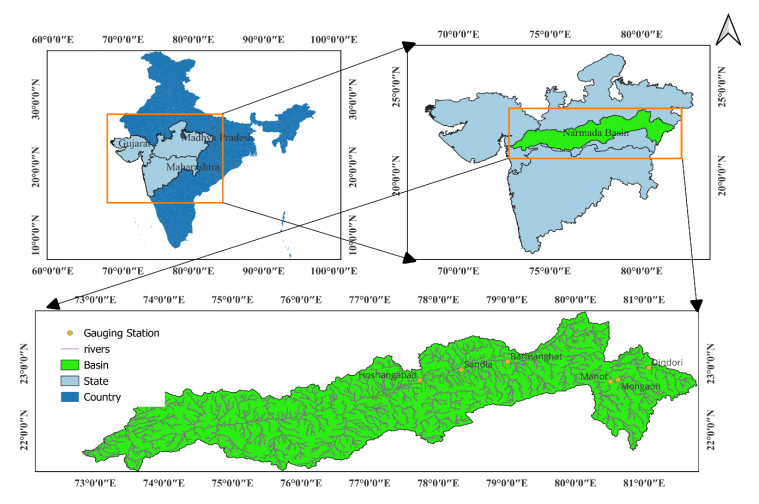
Accurate flood forecasting is a crucial process for predicting the timing, occurrence, duration, and magnitude of floods in specific zones. This prediction often involves analyzing various hydrological, meteorological, and environmental parameters. In recent years, several soft computing techniques have been widely used for flood forecasting. In this study, flood forecasting for the Narmada River at the Hoshangabad gauging site in Madhya Pradesh, India, was conducted using an Artificial Neural Network (ANN) model, a Fuzzy Logic (FL) model, and an Adaptive Neuro-Fuzzy Inference System (ANFIS) model. To assess their capacity to handle different levels of information, three separate input data sets were used. Our objective was to compare the performance and evaluate the suitability of soft computing data-driven models for flood forecasting. For the development of these models, monthly discharge data spanning 33 years from six gauging sites were selected. Various performance measures, such as regression, root mean square error (RMSE), and percentage deviation, were used to compare and evaluate the performances of the different models. The results indicated that the ANN and ANFIS models performed similarly in some cases. However, the ANFIS model generally predicted much better than the ANN model in most cases. The ANFIS model, developed using the hybrid method, delivered the best performance with an RMSE of 211.97 and a coefficient of regression of 0.96, demonstrating the potential of using these models for flood forecasting. This research highlighted the effectiveness of soft computing techniques in flood forecasting and established useful suitability criteria that can be employed by flood control departments in various countries, regions, and states for accurate flood prognosis.

Keywords:

Citation: Ronak P. Chaudhari, Shantanu R. Thorat, Darshan J. Mehta, Sahita I. Waikhom, Vipinkumar G. Yadav, Vijendra Kumar. Comparison of soft-computing techniques: Data-driven models for flood forecasting[J]. AIMS Environmental Science, 2024, 11(5): 741-758. doi: 10.3934/environsci.2024037

Related Papers:

[1]	Qun Dai, Shidong Liu . Stability of the mixed Caputo fractional integro-differential equation by means of weighted space method. AIMS Mathematics, 2022, 7(2): 2498-2511. doi: 10.3934/math.2022140
[2]	Thabet Abdeljawad, Sabri T. M. Thabet, Imed Kedim, Miguel Vivas-Cortez . On a new structure of multi-term Hilfer fractional impulsive neutral Levin-Nohel integrodifferential system with variable time delay. AIMS Mathematics, 2024, 9(3): 7372-7395. doi: 10.3934/math.2024357
[3]	Choukri Derbazi, Zidane Baitiche, Mohammed S. Abdo, Thabet Abdeljawad . Qualitative analysis of fractional relaxation equation and coupled system with Ψ-Caputo fractional derivative in Banach spaces. AIMS Mathematics, 2021, 6(3): 2486-2509. doi: 10.3934/math.2021151
[4]	J. Vanterler da C. Sousa, E. Capelas de Oliveira, F. G. Rodrigues . Ulam-Hyers stabilities of fractional functional differential equations. AIMS Mathematics, 2020, 5(2): 1346-1358. doi: 10.3934/math.2020092
[5]	Kaihong Zhao, Shuang Ma . Ulam-Hyers-Rassias stability for a class of nonlinear implicit Hadamard fractional integral boundary value problem with impulses. AIMS Mathematics, 2022, 7(2): 3169-3185. doi: 10.3934/math.2022175
[6]	Jiqiang Zhang, Siraj Ul Haq, Akbar Zada, Ioan-Lucian Popa . Stieltjes integral boundary value problem involving a nonlinear multi-term Caputo-type sequential fractional integro-differential equation. AIMS Mathematics, 2023, 8(12): 28413-28434. doi: 10.3934/math.20231454
[7]	Hasanen A. Hammad, Hassen Aydi, Hüseyin Işık, Manuel De la Sen . Existence and stability results for a coupled system of impulsive fractional differential equations with Hadamard fractional derivatives. AIMS Mathematics, 2023, 8(3): 6913-6941. doi: 10.3934/math.2023350
[8]	Dongming Nie, Usman Riaz, Sumbel Begum, Akbar Zada . A coupled system of $p$ -Laplacian implicit fractional differential equations depending on boundary conditions of integral type. AIMS Mathematics, 2023, 8(7): 16417-16445. doi: 10.3934/math.2023839
[9]	Thanin Sitthiwirattham, Rozi Gul, Kamal Shah, Ibrahim Mahariq, Jarunee Soontharanon, Khursheed J. Ansari . Study of implicit-impulsive differential equations involving Caputo-Fabrizio fractional derivative. AIMS Mathematics, 2022, 7(3): 4017-4037. doi: 10.3934/math.2022222
[10]	Subramanian Muthaiah, Dumitru Baleanu, Nandha Gopal Thangaraj . Existence and Hyers-Ulam type stability results for nonlinear coupled system of Caputo-Hadamard type fractional differential equations. AIMS Mathematics, 2021, 6(1): 168-194. doi: 10.3934/math.2021012

Abstract

1. Introduction

Fractional differential equations have played an important role and have presented valuable tools in the modeling of many phenomena in various fields of science and engineering ^{[6,7,8,9,10,11,12,13,14,15,16]}. There has been a significant development in fractional differential equations in recent decades ^{[2,3,4,5,26,23,33,37]}. On the other hand, many authors studied the stability of functional equations and established some types of Ulam stability ^{[1,17,18,19,20,21,22,24,27,28,29,30,31,32,33,34,35,36,37]} and references there in. Moreover, many authors discussed local and global attractivity ^{[8,9,10,11,34]}.

Benchohra et al. ^[13] established some types of Ulam-Hyers stability for an implicit fractional-order differential equation.

A. Baliki et al. ^[11] have given sufficient conditions for existence and attractivity of mild solutions for second order semi-linear functional evolution equation in Banach spaces using Schauder's fixed point theorem.

Benchohra et al. ^[15] studied the existence of mild solutions for a class of impulsive semilinear fractional differential equations with infinite delay and non-instantaneous impulses in Banach spaces. This results are obtained using the technique of measures of noncompactness.

Motivated by these works, in this paper, we investigate the following initial value problem for an implicit fractional-order differential equation

$\begin{align} \left\{ \begin{array}{c} ^C\mathfrak{D}^\alpha \left[ \mathfrak{x}(\mathfrak{t})- \mathfrak{h}(\mathfrak{t}, \mathfrak{x}(\mathfrak{t}))\right] = \mathfrak{g}_1( \mathfrak{t}, \mathfrak{x}(\mathfrak{t}), \mathfrak{I}^\mathfrak{\beta} \mathfrak{g}_2(\mathfrak{t}, \mathfrak{x}(\mathfrak{t}))) \; \; \; \mathfrak{t}\in {J}, \; 1 \lt \alpha \leq 2 , \; \alpha \geq \beta, \\\\ \bigg(\mathfrak{x}(\mathfrak{t})- \mathfrak{h}(\mathfrak{t}, \mathfrak{x}(t))\bigg)\bigg|_{\mathfrak{t} = 0} = 0\; \; \; \; \mbox{and}\; \; \; \; \; \frac{d}{d\mathfrak{t}}\big[\mathfrak{x}(\mathfrak{t})- \mathfrak{h}(\mathfrak{t}, \mathfrak{x}(\mathfrak{t}))\big]_{\mathfrak{t} = 0} = 0\end{array} \right. \end{align}$

(1.1)

where $\; ^C\mathfrak{D}^\alpha\;$ is the Caputo fractional derivative, $\; \mathfrak{h}:J \times R \longrightarrow R, \; \mathfrak{g} _{1}: J \times R \times R\longrightarrow R \;$ and $\mathfrak{g} _{2}:J \times R \longrightarrow R$ are given functions satisfy some conditions and $\; J = [0, T]$ .

we give sufficient conditions for the existence of solutions for a class of initial value problem for an neutral differential equation involving Caputo fractional derivatives. Also, we establish some types of Ulam-Hyers stability for this class of implicit fractional-order differential equation and some applications and particular cases are presented.

Finally, existence of at least one mild solution for this class of implicit fractional-order differential equation on an infinite interval $\; J = [0, +\infty), \;$ by applying Schauder fixed point theorem and proving the attractivity of these mild solutions.

By a solution of the Eq (1.1) we mean that a function $x \in C^2(J, R)$ such that

(i) the function $\mathfrak{t} \to \left[\mathfrak{x}(\mathfrak{t})- \mathfrak{h}(\mathfrak{t}, \mathfrak{x}(\mathfrak{t}))\right]\in C^2(J, R)$ and

(ii) $\mathfrak{x}$ satisfies the equation in (1.1).

2. Preliminaries

Definition 1. ^[23] The Riemann-Liouville fractional integral of the function $\mathfrak{f} \in L^1([\mathfrak{a}, \mathfrak{b}])$ of order $\alpha \in R_+$ is defined by

$\mathfrak{I}_{\mathfrak{a}}^{\alpha}\; \mathfrak{f}(\mathfrak{t}) = \int_{\mathfrak{a}}^\mathfrak{t}\; \frac{(\mathfrak{t}-\mathfrak{s})^{\alpha-1}}{\Gamma(\alpha)} \; \mathfrak{f}(\mathfrak{s}) \; d\mathfrak{s}.$

and when $\mathfrak{a} = 0,$ we have $\mathfrak{I}^{\alpha}\; \mathfrak{f}(\mathfrak{t}) = \mathfrak{I}_{0}^{\alpha}\; \mathfrak{f}(\mathfrak{t}).$

Definition 2. ^[23] For a function $\; \mathfrak{f}:[\mathfrak{a}, \mathfrak{b}]\rightarrow R\;$ the Caputo fractional-order derivative of $\; \mathfrak{f}, \;$ is defined by

$^C\mathfrak{D}^\alpha \mathfrak{h}(\mathfrak{t}) = \frac{1}{\Gamma(\mathfrak{n}-\alpha)}\int_\mathfrak{a}^\mathfrak{t} \frac{\mathfrak{h}^{(\mathfrak{n})}(\mathfrak{s})}{(\mathfrak{t}-\mathfrak{s})^{\mathfrak{n}-\alpha-1}}\; d\mathfrak{s},$

where where $\; \mathfrak{n} = [\alpha]+ 1\;$ and $\; [\alpha]\;$ denotes the integer part of the real number $\; \alpha.$

Lemma 1. ^[23]. Let $\; \alpha \geq 0\;$ and $\; \mathfrak{n} = [\alpha]+ 1.\;$ Then

$\mathfrak{I}^\alpha(^C\mathfrak{D}^\alpha \mathfrak{f}(\mathfrak{t})) = \mathfrak{f}(\mathfrak{t})- \sum\limits_{k = 0}^{\mathfrak{n}-1}\frac{\mathfrak{f}^k(0)}{k!}\mathfrak{t}^k$

Lemma 2. Let $\; \mathfrak{f} \in L^1([\mathfrak{a}, \mathfrak{b}])\;$ and $\; \alpha \in (0, 1], \;$ then

(i) $^C\mathfrak{D}^{\alpha}\mathfrak{I}^\alpha \mathfrak{f}(\mathfrak{t}) = \mathfrak{f}(\mathfrak{t}).\; \;$

(ii) The operator $\; \mathfrak{I}^\alpha\;$ maps $\; L^1([\mathfrak{a}, \mathfrak{b}])\;$ into itself continuously.

(iii) For $\; \gamma, \; \beta > 0, \;$ then

$\mathfrak{I}_\mathfrak{a}^\beta \; \mathfrak{I}_\mathfrak{a}^\gamma \; \mathfrak{f}(\mathfrak{t})\; = \; \mathfrak{I}_\mathfrak{a}^\gamma \mathfrak{I}_\mathfrak{a}^\beta \; \mathfrak{f}(\mathfrak{t})\; = \; \mathfrak{I}_\mathfrak{a}^{\gamma+\beta}\; \mathfrak{f}(\mathfrak{t}),$

For further properties of fractional operators (see ^[23,25,26]).

3. Main results

Consider the initial value problem for the implicit fractional-order differential Eq (1.1) under the following assumptions:

(i) $\mathfrak{h}:J \times R \longrightarrow R$ is a continuous function and there exists a positive constant $K_1$ such that:

$\mid \mathfrak{h}(\mathfrak{t}, \mathfrak{x})- \mathfrak{h}(\mathfrak{t}, \mathfrak{y})\mid \leqslant K_1 \mid \mathfrak{x}-\mathfrak{y}\mid \; \; \mbox{ for each }\; \; \mathfrak{t}\in J \; \mbox{ and } \; \mathfrak{x}, \mathfrak{y}\in R.$

(ii) $\mathfrak{g} _{1}: J \times R \times R\longrightarrow R$ is a continuous function and there exist two positive constants $K, H$ such that:

$\mid \mathfrak{g} _{1}(\mathfrak{t}, \mathfrak{x}, \mathfrak{y}) - \mid \mathfrak{g} _{1}(\mathfrak{t}, \widetilde{\mathfrak{x}}, \widetilde{\mathfrak{y}}) \mid \leqslant K \mid \mathfrak{x}- \widetilde{\mathfrak{x}} \mid + H \mid \mathfrak{y}- \widetilde{\mathfrak{y}}\mid \; \mbox{ for each }\; \mathfrak{t}\in J \; \mbox{ and }\; \mathfrak{x}, \widetilde{\mathfrak{x}}, \mathfrak{y}, \widetilde{\mathfrak{y}} \in R$

(iii) $\mathfrak{g }_{2}:J \times R \longrightarrow R$ is a continuous function and there exists a positive constant $K_2$ such that:

$\mid \mathfrak{g}_2(\mathfrak{t}, \mathfrak{x})- \mathfrak{g}_2(\mathfrak{t}, \mathfrak{y})\mid \leqslant K_2 \mid \mathfrak{x}-\mathfrak{y}\mid \; \mbox{ for each } \; \mathfrak{t}\in J \; \mbox{ and} \; \mathfrak{x}, \mathfrak{y}\in R.$

Lemma 3. Let assumptions (i)-(iii) be satisfied. If a function $\mathfrak{x} \in C^2(J, R)$ is a solution of initial value problem for implicit fractional-order differential equation $(1.1)$ , then it is a solution of the following nonlinear fractional integral equation

$\begin{equation} \mathfrak{x}(\mathfrak{t}) = \mathfrak{h}(\mathfrak{t}, \mathfrak{x}(\mathfrak{t}))+\frac{1}{\Gamma(\alpha)}\int_0^\mathfrak{t}(\mathfrak{t}-\mathfrak{s})^{\alpha-1}\mathfrak{g}_1\left(\mathfrak{s}, \mathfrak{x}(\mathfrak{s}), \frac{1}{\Gamma(\beta)}\int_0^\mathfrak{s}(\mathfrak{s}-\theta)^{\beta-1}\mathfrak{g}_2(\theta, \mathfrak{x}(\theta))d\theta\right)d\mathfrak{s} \end{equation}$

(3.1)

Proof. Assume first that $\mathfrak{x}$ is a solution of the initial value problem (1.1). From definition of Caputo derivative, we have

$\mathfrak{I}^{2-\alpha}\mathfrak{D}^2\left(\mathfrak{x}(\mathfrak{t})- \mathfrak{h}(\mathfrak{t}, \mathfrak{x}(\mathfrak{t}))\right) = \mathfrak{g}_1( \mathfrak{t}, \mathfrak{x}(\mathfrak{t}), \mathfrak{I}^\beta \mathfrak{g}_2(\mathfrak{t}, \mathfrak{x}(\mathfrak{t}))).$

Operating by $\; \mathfrak{I}^{\alpha-1}\;$ on both sides and using Lemma 2, we get

$\mathfrak{I}^{1}\mathfrak{D}^2\left(\mathfrak{x}(\mathfrak{t})- \mathfrak{h}(\mathfrak{t}, \mathfrak{x}(\mathfrak{t}))\right) = \mathfrak{I}^{\alpha-1}\mathfrak{g}_1( \mathfrak{t}, \mathfrak{x}(\mathfrak{t}), \mathfrak{I}^\beta \mathfrak{g}_2(\mathfrak{t}, \mathfrak{x}(\mathfrak{t}))).$

Then

$\frac{d}{d\mathfrak{t}}\big(\mathfrak{x}(\mathfrak{t})- \mathfrak{h}(\mathfrak{t}, \mathfrak{x}(\mathfrak{t}))\big)- \frac{d}{d\mathfrak{t}}\big(\mathfrak{x}(\mathfrak{t})- \mathfrak{h}(\mathfrak{t}, \mathfrak{x}(\mathfrak{t}))\big)\bigg|_{\mathfrak{t} = 0} = \mathfrak{I}^{\alpha-1}\mathfrak{g}_1( \mathfrak{t}, \mathfrak{x}(\mathfrak{t}), \mathfrak{I}^\beta \mathfrak{g}_2(\mathfrak{t}, \mathfrak{x}(\mathfrak{t}))).$

Using initial conditions, we have

$\frac{d}{d\mathfrak{t}}\big(\mathfrak{x}(\mathfrak{t})- \mathfrak{h}(\mathfrak{t}, \mathfrak{x}(\mathfrak{t}))\big) = \mathfrak{I}^{\alpha-1}\mathfrak{g}_1( \mathfrak{t}, \mathfrak{x}(\mathfrak{t}), \mathfrak{I}^\beta \mathfrak{g}_2(\mathfrak{t}, \mathfrak{x}(\mathfrak{t}))).$

Integrating both sides of (1.1), we obtain

$\big(\mathfrak{x}(\mathfrak{t})- \mathfrak{h}(\mathfrak{t}, \mathfrak{x}(\mathfrak{t}))\big)-\big(\mathfrak{x}(\mathfrak{t})- \mathfrak{h}(\mathfrak{t}, \mathfrak{x}(\mathfrak{t}))\big)\bigg|_{\mathfrak{t} = 0} = \mathfrak{I}^{\alpha}\mathfrak{g}_1( \mathfrak{t}, \mathfrak{x}(\mathfrak{t}), \mathfrak{I}^\beta \mathfrak{g}_2(\mathfrak{t}, \mathfrak{x}(\mathfrak{t}))).$

Then

$\mathfrak{x}(\mathfrak{t}) = \mathfrak{h}(\mathfrak{t}, \mathfrak{x}(\mathfrak{t}))+\frac{1}{\Gamma(\alpha)}\int_0^\mathfrak{t}(\mathfrak{t}-\mathfrak{s})^{\alpha-1}\mathfrak{g}_1\left(\mathfrak{s}, \mathfrak{x}(\mathfrak{s}), \frac{1}{\Gamma(\beta)}\int_0^\mathfrak{s}(\mathfrak{s}-\theta)^{\beta-1}\mathfrak{g}_2(\theta, \mathfrak{x}(\theta))d\theta\right)d\mathfrak{s}$

Conversely, assume that $\mathfrak{x}$ satisfies the nonlinear integral Eq (3.1). Then operating by $\; ^C\mathfrak{D}^\alpha \;$ on both sides of Eq (3.1) and using Lemma 2, we obtain

$\begin{eqnarray*} ^C\mathfrak{D}^\alpha \big(\mathfrak{x}(\mathfrak{t})-\mathfrak{h}(\mathfrak{t}, \mathfrak{x}(\mathfrak{t}))\big) & = &^C\mathfrak{D}^\alpha \mathfrak{I}^\alpha \mathfrak{g}_1( \mathfrak{t}, \mathfrak{x}(\mathfrak{t}), \mathfrak{I}^\beta \mathfrak{g}_2(\mathfrak{t}, \mathfrak{x}(\mathfrak{t})))\\ & = &\mathfrak{g}_1( \mathfrak{t}, \mathfrak{x}(\mathfrak{t}), \mathfrak{I}^\beta \mathfrak{g}_2(\mathfrak{t}, \mathfrak{x}(\mathfrak{t}))). \end{eqnarray*}$

Putting $\mathfrak{t} = 0$ in (3.1) and since $\; \mathfrak{g}_1\;$ is a continuous function, then we obtain

$\big(\mathfrak{x}(\mathfrak{t})-\mathfrak{h}(\mathfrak{t}, \mathfrak{x}(\mathfrak{t}))\big)\bigg|_{\mathfrak{t} = 0} = I^\alpha \mathfrak{g}_1( \mathfrak{t}, \mathfrak{x}(\mathfrak{t}), \mathfrak{I}^\beta \mathfrak{g}_2(\mathfrak{t}, \mathfrak{x}(\mathfrak{t})))\bigg|_{\mathfrak{t} = 0} = 0.$

Also,

Then we have

$\frac{d}{d\mathfrak{t}}\big(\mathfrak{x}(\mathfrak{t})- \mathfrak{h}(\mathfrak{t}, \mathfrak{x}(\mathfrak{t}))\big)\bigg|_{\mathfrak{t} = 0} = \mathfrak{I}^{\alpha-1}\mathfrak{g}_1( \mathfrak{t}, \mathfrak{x}(\mathfrak{t}), \mathfrak{I}^\beta \mathfrak{g}_2(\mathfrak{t}, \mathfrak{x}(\mathfrak{t})))\bigg|_{\mathfrak{t} = 0} = 0.$

Hence the equivalence between the initial value problem (1.1) and the integral Eq (3.1) is proved. Then the proof is completed.

Definition 3. The Eq (1.1) is Ulam-Hyers stable if there exists a real number $\mathfrak{c}_{\mathfrak{f}} > 0$ such that for each $\epsilon > 0$ and for each solution $\mathfrak{z}\in C^{2}(J, R)$ of the inequality

$\mid ^C\mathfrak{D}^\alpha \left[ \mathfrak{z}(\mathfrak{t})- \mathfrak{h}(\mathfrak{t}, \mathfrak{z}(\mathfrak{t}))\right] - \mathfrak{g}_1( \mathfrak{t}, \mathfrak{z}(\mathfrak{t}), \mathfrak{I}^\beta\mathfrak{ g}_2(\mathfrak{t}, \mathfrak{z}(\mathfrak{t}))) \mid \leqslant \epsilon, \; \mathfrak{t}\in J,$

there exists a solution $\mathfrak{y}\in C^{2}(J, R)$ of Eq (1.1) with

$\mid \mathfrak{z}(\mathfrak{t})-\mathfrak{y}(\mathfrak{t})\vert \leqslant \mathfrak{c}_{\mathfrak{f}}\epsilon, \; \mathfrak{t}\in J .$

Definition 4. The Eq (1.1) is generalized Ulam-Hyers stable if there exists $\psi_{\mathfrak{f}}\in C(R_{+}, R_{+}), \; \psi_{\mathfrak{f}}(0) = 0,$ such that for each solution $\mathfrak{z}\in C^{2}(J, R)$ of the inequality

$\mid ^C\mathfrak{D}^\alpha \left[ \mathfrak{z}(\mathfrak{t})- \mathfrak{h}(\mathfrak{t}, \mathfrak{z}(\mathfrak{t}))\right] - \mathfrak{g}_1( \mathfrak{t}, \mathfrak{z}(\mathfrak{t}), \mathfrak{I}^\beta \mathfrak{g}_2(\mathfrak{t}, \mathfrak{z}(\mathfrak{t}))) \mid \leqslant \epsilon , \; \mathfrak{t}\in J,$

there exists a solution $\mathfrak{y}\in C^{2}(J, R)\;$ of Eq (1.1) with

$\mid \mathfrak{z}(\mathfrak{t})-\mathfrak{y}(\mathfrak{t})\vert \leqslant \psi_{\mathfrak{f}} (\epsilon), \; \mathfrak{t}\in J .$

Definition 5. The Eq (1.1) is Ulam-Hyers-Rassias stable with respect to $\varphi\in C(J, R_{+})$ if there exists a real number $\mathfrak{c}_{\mathfrak{f}} > 0$ such that for each $\epsilon > 0$ and for each solution $\mathfrak{z}\in C^{2}(J, R)$ of the inequality

$\mid ^C\mathfrak{D}^\alpha \left[ \mathfrak{z}(\mathfrak{t})-\mathfrak{ h}(\mathfrak{t}, \mathfrak{z}(\mathfrak{t}))\right] - \mathfrak{g}_1( \mathfrak{t}, \mathfrak{z}(\mathfrak{t}), \mathfrak{I}^\beta \mathfrak{g}_2(\mathfrak{t}, \mathfrak{z}(\mathfrak{t}))) \mid \leqslant \epsilon \varphi(\mathfrak{t}) , \; \mathfrak{t}\in J,$

there exists a solution $\mathfrak{y}\in C^{2}(J, R)$ of Eq (1.1) with

$\mid \mathfrak{z}(\mathfrak{t})-\mathfrak{y}(\mathfrak{t})\vert \leqslant \mathfrak{c}_\mathfrak{f}\epsilon\varphi(\mathfrak{t}), \; \mathfrak{t}\in J.$

Definition 6. The Eq (1.1) is generalized Ulam-Hyers-Rassias stable with respect to $\varphi\in C(J, R_{+})$ if there exists a real number $\mathfrak{c}_{\mathfrak{f}, \varphi} > 0$ such that for each solution $\mathfrak{z}\in C^{2}(J, R)$ of the inequality

$\mid ^C\mathfrak{D}^\alpha \left[ \mathfrak{z}(\mathfrak{t})- \mathfrak{h}(\mathfrak{t}, \mathfrak{z}(\mathfrak{t}))\right] - \mathfrak{g}_1( \mathfrak{t}, \mathfrak{z}(\mathfrak{t}), \mathfrak{I}^\beta \mathfrak{g}_2(\mathfrak{t}, \mathfrak{z}(\mathfrak{t}))) \mid \leqslant \varphi(\mathfrak{t}) , \; \mathfrak{t}\in J,$

there exists a solution $\mathfrak{y}\in C^{2}(J, R)$ of Eq (1.1) with

$\mid \mathfrak{z}(\mathfrak{t})-\mathfrak{y}(\mathfrak{t})\vert \leqslant \mathfrak{c}_{\mathfrak{f}, \varphi} \varphi (\mathfrak{t}) , \; \mathfrak{t}\in J.$

Now, our aim is to investigate the existence of unique solution for (1.1). This existence result will be based on the contraction mapping principle.

Theorem 1. Let assumptions (i)-(iii) be satisfied. If $\; K_1+ \dfrac{K\; T^\alpha}{\Gamma(\alpha+1)}+\dfrac{K_2\; H\; T^{\alpha+\beta}}{\Gamma(\beta+1)\Gamma(\alpha+1)} < 1, \;$ then there exists a unique solution for the nonlinear neutral differential equation of fractional order.

Proof. Define the operator $\; N\;$ by:

$N\mathfrak{x}(\mathfrak{t}) = \mathfrak{h}(\mathfrak{t}, \mathfrak{x}(\mathfrak{t}))+\frac{1}{\Gamma(\alpha)}\int_0^\mathfrak{t}(\mathfrak{t}-\mathfrak{s})^{\alpha-1}\mathfrak{g}_1\left(\mathfrak{s}, \mathfrak{x}(\mathfrak{s}), \frac{1}{\Gamma(\beta)}\int_0^\mathfrak{s}(\mathfrak{s}-\theta)^{\beta-1}\mathfrak{g}_2(\theta, \mathfrak{x}(\theta))d\theta\right)d\mathfrak{s}, \; \mathfrak{t}\in J.$

In view of assumptions (i)-(iii), then $\; N: C^2(J, R) \rightarrow C^2(J, R)\;$ is continuous operator.

Now, let $\mathfrak{x}$ and $, \widetilde{\mathfrak{x}} \in C^2(J, R), \;$ be two solutions of (1.1)then

$\begin{eqnarray*} \mid N\mathfrak{x}(\mathfrak{t})-N\widetilde{\mathfrak{x}}(\mathfrak{t})\mid& = & \bigg| \mathfrak{h}(\mathfrak{t}, \mathfrak{x}(\mathfrak{t}))\\ &+&\dfrac{1}{\Gamma(\alpha)}\int_{0}^{\mathfrak{t}} (\mathfrak{t}-\mathfrak{s})^{\alpha-1}\mathfrak{g}_{1}\bigg(\mathfrak{s}, \mathfrak{x}(\mathfrak{s}), \dfrac{1}{\Gamma(\beta)}\int_{0}^{\mathfrak{s}} (\mathfrak{s}-\theta)^{\beta-1}\mathfrak{g}_{2}(\theta, \mathfrak{x}(\theta))d\theta\bigg)d\mathfrak{s}\\ \; \; \; \; \; \; &-&\mathfrak{h}(\mathfrak{t}, \widetilde{\mathfrak{x}}(\mathfrak{t}))\\ &-&\dfrac{1}{\Gamma(\alpha)}\int_{0}^{\mathfrak{t}} (\mathfrak{t}-\mathfrak{s})^{\alpha-1}\mathfrak{g}_{1}\bigg(\mathfrak{s}, \widetilde{\mathfrak{x}}(\mathfrak{s}), \dfrac{1}{\Gamma(\beta)}\int_{0}^{\mathfrak{s}} (\mathfrak{s}-\theta)^{\beta-1}\mathfrak{g}_{2}(\theta, \widetilde{\mathfrak{x}}(\theta))d\theta\bigg)d\mathfrak{s}\bigg|\\ &\leqslant& K_1|\mathfrak{x}(\mathfrak{t})-\widetilde{\mathfrak{x}}(\mathfrak{t})|\\ &+& \dfrac{1}{\Gamma(\alpha)}\int_{0}^{\mathfrak{t}} (\mathfrak{t}-\mathfrak{s})^{\alpha-1}\bigg| \mathfrak{g}_{1}\bigg(\mathfrak{s}, \mathfrak{x}(\mathfrak{s}), \dfrac{1}{\Gamma(\beta)}\int_{0}^{\mathfrak{s}} (\mathfrak{s}-\theta)^{\beta-1}\mathfrak{g}_{2}(\theta, \mathfrak{x}(\theta))d\theta\bigg)\\ \; \; \; \; \; \; &-& g_{1}\bigg(\mathfrak{s}, \widetilde{\mathfrak{x}}(\mathfrak{s}), \dfrac{1}{\Gamma(\beta)}\int_{0}^{\mathfrak{s}} (\mathfrak{s}-\theta)^{\beta-1}\mathfrak{g}_{2}(\theta, \widetilde{\mathfrak{x}}(\theta))d\theta\bigg)\bigg| d\mathfrak{s}\\ \; \; \; \; \; \; &\leqslant&K_1|\mathfrak{x}(\mathfrak{t})-\widetilde{\mathfrak{x}}(\mathfrak{t})|\\ &+& \dfrac{1}{\Gamma(\alpha)}\int_{0}^{\mathfrak{t}} (\mathfrak{t}-\mathfrak{s})^{\alpha-1} K\mid \mathfrak{x}(\mathfrak{s})-\widetilde{\mathfrak{x}}(\mathfrak{s})\vert d\mathfrak{s} \\ &+&H\dfrac{1}{\Gamma(\alpha)}\int_{0}^{\mathfrak{t}} (\mathfrak{t}-\mathfrak{s})^{\alpha-1} \dfrac{1}{\Gamma(\beta)}\int_{0}^{\mathfrak{s}} (\mathfrak{s}-\theta)^{\beta-1}\mid \mathfrak{g}_{2}(\theta, \mathfrak{x}(\theta))- \mathfrak{g}_{2}(\theta, \widetilde{\mathfrak{x}}(\theta))\vert d\theta d\mathfrak{s}\\ \; \; \; \; \; \; &\leqslant&K_1|\mathfrak{x}(\mathfrak{t})-\widetilde{\mathfrak{x}}(\mathfrak{t})|+ \dfrac{K}{\Gamma(\alpha)}\int_{0}^{\mathfrak{t}} (\mathfrak{t}-\mathfrak{s})^{\alpha-1} \mid \mathfrak{x}(\mathfrak{s})-\widetilde{\mathfrak{x}}(\mathfrak{s})\vert d\mathfrak{s} \\ &+& \dfrac{H}{\Gamma(\alpha)}\int_{0}^{\mathfrak{t}} (\mathfrak{t}-\mathfrak{s})^{\alpha-1}\dfrac{K_2}{\Gamma(\beta)}\int_{0}^{\mathfrak{s}} (\mathfrak{s}-\theta)^{\beta-1}\mid \mathfrak{x}(\theta)- \widetilde{\mathfrak{x}}(\theta)\vert d\theta d\mathfrak{s}. \end{eqnarray*}$

Then

$\begin{eqnarray*} || N\mathfrak{x}(\mathfrak{t})-N\widetilde{\mathfrak{x}}(\mathfrak{t})||&\leqslant&K_1||\mathfrak{x}-\widetilde{\mathfrak{x}}||+ \dfrac{K|| \mathfrak{x}-\widetilde{\mathfrak{x}}|\vert}{\Gamma(\alpha)}\int_{0}^{\mathfrak{t}} (\mathfrak{t}-\mathfrak{s})^{\alpha-1} d\mathfrak{s} \\ &+& || \mathfrak{x}- \widetilde{\mathfrak{x}}\vert| \dfrac{H}{\Gamma(\alpha)}\int_{0}^{\mathfrak{t}} (\mathfrak{t}-\mathfrak{s})^{\alpha-1}\dfrac{K_2}{\Gamma(\beta)}\int_{0}^{\mathfrak{s}} (\mathfrak{s}-\theta)^{\beta-1} d\theta d\mathfrak{s}\\ &\leqslant&K_1||\mathfrak{x}-\widetilde{\mathfrak{x}}||+ \dfrac{K|| \mathfrak{x}-\widetilde{\mathfrak{x}}|\vert\; T^\alpha}{\Gamma(\alpha+1)} \\ &+& || \mathfrak{x}- \widetilde{\mathfrak{x}}\vert|\dfrac{K_2\; T^\beta}{\Gamma(\beta+1)} \dfrac{H}{\Gamma(\alpha)}\int_{0}^{\mathfrak{t}} (\mathfrak{t}-\mathfrak{s})^{\alpha-1} d\mathfrak{s}\\ &\leqslant&K_1||\mathfrak{x}-\widetilde{\mathfrak{x}}||+ \dfrac{K|| \mathfrak{x}-\widetilde{\mathfrak{x}}|\vert\; T^\alpha}{\Gamma(\alpha+1)} \\ &+& || \mathfrak{x}- \widetilde{\mathfrak{x}}\vert|\dfrac{K_2\; T^\beta}{\Gamma(\beta+1)} \dfrac{H\; T^\alpha}{\Gamma(\alpha+1)}\\ &\leq& \left[K_1+ \dfrac{K\; T^\alpha}{\Gamma(\alpha+1)}+\dfrac{K_2\; H\; T^{\alpha+\beta}}{\Gamma(\beta+1)\Gamma(\alpha+1)} \right]|| \mathfrak{x}-\widetilde{\mathfrak{x}}|\vert \end{eqnarray*}$

Since $\; K_1+ \dfrac{K\; T^\alpha}{\Gamma(\alpha+1)}+\dfrac{K_2\; H\; T^{\alpha+\beta}}{\Gamma(\beta+1)\Gamma(\alpha+1)} < 1. \;$ It follows that $N$ has a unique fixed point which is a solution of the initial value problem (1.1) in $\; C^2(J, R).\;$

4. Stability of solutions of the IVP (1.1)

4.1. Ulam-Hyers stability

Theorem 2. Let assumptions of Theorem 1 be satisfied. Then the fractional order differential Eq (1.1) is Ulam-Hyers stable.

Proof. Let $\; \mathfrak{y}\in C^2(J, R)\;$ be a solution of the inequality

$\begin{equation} \mid ^C\mathfrak{D}^\alpha \left[ \mathfrak{y}(\mathfrak{t})- \mathfrak{h}(\mathfrak{t}, \mathfrak{y}(\mathfrak{t}))\right] - \mathfrak{g}_1( \mathfrak{t}, \mathfrak{y}(\mathfrak{t}), \mathfrak{I}^\beta\mathfrak{ g}_2(\mathfrak{t}, \mathfrak{y}(\mathfrak{t}))) \mid \leqslant \epsilon, \; \epsilon \gt 0, \; \mathfrak{t}\in J. \end{equation}$

(4.1)

Let $\; \mathfrak{x}\in C^2(J, R)\;$ be the unique solution of the initial value problem for implicit fractional-order differential Eq (1.1). By using Lemma 3, The Cauchy problem (1.1) is equivalent to

Operating by $\; \mathfrak{I}^{\alpha-1}\;$ on both sides of (4.1) and then integrating, we get

$\begin{eqnarray*} \bigg| \mathfrak{y}(\mathfrak{t})-\mathfrak{h}(\mathfrak{t}, \mathfrak{y}(\mathfrak{t}))&-&\frac{1}{\Gamma(\alpha)}\int_0^\mathfrak{t} (\mathfrak{t}-\mathfrak{s})^{\alpha-1}\mathfrak{g}_1\left(\mathfrak{s}, \mathfrak{y}(\mathfrak{s}), \frac{1}{\Gamma(\beta)}\int_0^\mathfrak{s}(\mathfrak{s}-\theta)^{\beta-1}\mathfrak{g}_2(\theta, \mathfrak{y}(\theta))d\theta\right)d\mathfrak{s}\bigg| \\ &\leqslant& \frac{1}{\Gamma(\alpha)}\int_0^\mathfrak{t}(\mathfrak{t}-\mathfrak{s})^{\alpha-1}\epsilon \; d\mathfrak{s}, \\ &\leq & \frac{\epsilon\; T^\alpha}{\Gamma(\alpha+1)}. \end{eqnarray*}$

Also, we have

$\begin{eqnarray*} |\mathfrak{\mathfrak{y}}(\mathfrak{\mathfrak{t}})-\mathfrak{\mathfrak{x}}(\mathfrak{t})|& = & \bigg|\mathfrak{y}(\mathfrak{t})-\mathfrak{h}(\mathfrak{t}, \mathfrak{x}(\mathfrak{t}))-\frac{1}{\Gamma(\alpha)}\int_0^\mathfrak{t}(\mathfrak{t}-\mathfrak{s})^{\alpha-1}\mathfrak{g}_1\left(\mathfrak{s}, \mathfrak{x}(\mathfrak{s}), \frac{1}{\Gamma(\beta)}\int_0^\mathfrak{s}(\mathfrak{s}-\theta)^{\beta-1}\mathfrak{g}_2(\theta, \mathfrak{ x}(\theta))d\theta\right)d\mathfrak{s}\bigg|\\ & = &\bigg|\mathfrak{y}(\mathfrak{t})-\mathfrak{h}(\mathfrak{t}, \mathfrak{x}(\mathfrak{t}))-\frac{1}{\Gamma(\alpha)}\int_0^\mathfrak{t}(\mathfrak{t}-\mathfrak{s})^{\alpha-1}\mathfrak{g}_1\left(\mathfrak{s}, \mathfrak{x}(\mathfrak{s}), \frac{1}{\Gamma(\beta)}\int_0^\mathfrak{s}(\mathfrak{s}-\theta)^{\beta-1}\mathfrak{g}_2(\theta, \mathfrak{x}(\theta))d\theta\right)d\mathfrak{s}\\ &+& \mathfrak{h}(\mathfrak{t}, \mathfrak{y}(\mathfrak{t}))+\frac{1}{\Gamma(\alpha)}\int_0^\mathfrak{t}(\mathfrak{t}-\mathfrak{s})^{\alpha-1}\mathfrak{g}_1\left(\mathfrak{s}, \mathfrak{y}(\mathfrak{s}), \frac{1}{\Gamma(\beta)}\int_0^\mathfrak{s}(\mathfrak{s}-\theta)^{\beta-1}\mathfrak{g}_2(\theta, \mathfrak{y}(\theta))d\theta\right)d\mathfrak{s}\\ &-& \mathfrak{h}(\mathfrak{t}, \mathfrak{y}(\mathfrak{t}))-\frac{1}{\Gamma(\alpha)}\int_0^\mathfrak{t}(\mathfrak{t}-\mathfrak{s})^{\alpha-1}\mathfrak{g}_1\left(\mathfrak{s}, \mathfrak{y}(\mathfrak{s}), \frac{1}{\Gamma(\beta)}\int_0^\mathfrak{s}(\mathfrak{s}-\theta)^{\beta-1}\mathfrak{g}_2(\theta, \mathfrak{y}(\theta))d\theta\right)d\mathfrak{s}\bigg|\\ &\leq& \bigg|\mathfrak{y}(\mathfrak{t})-\mathfrak{h}(\mathfrak{t}, \mathfrak{y}(\mathfrak{t}))-\frac{1}{\Gamma(\alpha)}\int_0^\mathfrak{t}(\mathfrak{t}-\mathfrak{s})^{\alpha-1}\mathfrak{g}_1\left(\mathfrak{s}, \mathfrak{y}(\mathfrak{s}), \frac{1}{\Gamma(\beta)}\int_0^\mathfrak{s}(\mathfrak{s}-\theta)^{\beta-1}\mathfrak{g}_2(\theta, \mathfrak{ y}(\theta))d\theta\right)d\mathfrak{s}\bigg|\\ &+& | \mathfrak{h}(\mathfrak{t}, \mathfrak{y}(\mathfrak{t}))-\mathfrak{h}(\mathfrak{t}, \mathfrak{x}(\mathfrak{t}))| \\ &+&\frac{1}{\Gamma(\alpha)}\int_0^\mathfrak{t}(\mathfrak{t}-\mathfrak{s})^{\alpha-1} \bigg|\mathfrak{g}_1\left(\mathfrak{s}, \mathfrak{y}(\mathfrak{s}), \frac{1}{\Gamma(\beta)}\int_0^\mathfrak{s}(\mathfrak{s}-\theta)^{\beta-1}\mathfrak{g}_2(\theta, \mathfrak{y}(\theta))d\theta\right)\\ &-&\mathfrak{g}_1\left(\mathfrak{s}, \mathfrak{x}(\mathfrak{s}), \frac{1}{\Gamma(\beta)}\int_0^\mathfrak{s}(\mathfrak{s}-\theta)^{\beta-1}\mathfrak{g}_2(\theta, \mathfrak{x}(\theta))d\theta\right)\bigg|d\mathfrak{s}\\ &\leq& \frac{\epsilon\; T^\alpha}{\Gamma(\alpha+1)}+K_1|\mathfrak{y}(\mathfrak{t})-\mathfrak{x}(\mathfrak{t})|\\ &+&\frac{1}{\Gamma(\alpha)}\int_0^\mathfrak{t}(\mathfrak{t}-\mathfrak{s})^{\alpha-1} \left[K|\mathfrak{y}(\mathfrak{t})-\mathfrak{x}(\mathfrak{t})|+\frac{H}{\Gamma(\beta)}\int_0^\mathfrak{s}(\mathfrak{s}-\theta)^{\beta-1}|\mathfrak{g}_2(\theta, \mathfrak{y}(\theta))-\mathfrak{g}_2(\theta, \mathfrak{x}(\theta))|d\theta\right]d\mathfrak{s} \end{eqnarray*}$

$\begin{eqnarray*} ||\mathfrak{y}-\mathfrak{x}||&\leq& \frac{\epsilon \; T^\alpha}{\Gamma(\alpha+1)}+K_1||\mathfrak{y}-\mathfrak{x}||\\ &+&\frac{1}{\Gamma(\alpha)}\int_0^\mathfrak{t}(\mathfrak{t}-\mathfrak{s})^{\alpha-1} \left[K||\mathfrak{y}-\mathfrak{x}||+\frac{H\; K_2||\mathfrak{x}-\mathfrak{y}||T^\beta}{\Gamma(\beta+1)}\right]d\mathfrak{s}\\ &\leq& \frac{\epsilon\; T^\alpha}{\Gamma(\alpha+1)}+K_1||\mathfrak{y}-\mathfrak{x}||\\ &+&\frac{K\; T^\alpha||\mathfrak{y}-\mathfrak{x}||}{\Gamma(\alpha+1)} +\frac{H\; K_2T^{\beta+\alpha} ||\mathfrak{x}-\mathfrak{y}||}{\Gamma(\beta+1)\Gamma(\alpha+1)}. \end{eqnarray*}$

Then

$||\mathfrak{y}-\mathfrak{x}||\leq \frac{\epsilon \; T^\alpha}{\Gamma(\alpha+1)}\left[1- \left( K_1+\frac{K\; T^\alpha}{\Gamma(\alpha+1)} +\frac{H\; K_2\; T^{\beta+\alpha} }{\Gamma(\beta+1)\Gamma(\alpha+1)}\right)\right]^{-1} = \mathfrak{c}\; \epsilon,$

thus the intial value problem (1.1) is Ulam-Heyers stable, and hence the proof is completed. By putting $\psi(\varepsilon) = \mathfrak{c}\; \varepsilon, \; \psi(0) = 0 \;$ yields that the Eq (1.1) is generalized Ulam-Heyers stable.

4.2. Ulam-Hyers-Rassias stability

Theorem 3. Let assumptions of Theorem 1 be satisfied, there exists an increasing function $\varphi\in C(J, R)$ and there exists $\lambda_{\varphi} > 0$ such that for any $\mathfrak{t}\in J,$ we have

$\mathfrak{I}^{\alpha} \varphi (\mathfrak{t})\leqslant \lambda_{\varphi} \varphi(\mathfrak{t}),$

then the Eq (1.1) is Ulam-Heyers-Rassias stable.

Proof. Let $\; \mathfrak{y}\in C^2(J, R)\;$ be a solution of the inequality

$\begin{equation} \mid ^C\mathfrak{D}^\alpha \left[ \mathfrak{y}(\mathfrak{t})- \mathfrak{h}(\mathfrak{t}, \mathfrak{y}(\mathfrak{t}))\right] - \mathfrak{g}_1( \mathfrak{t}, \mathfrak{y}(\mathfrak{t}), \mathfrak{I}^\beta \mathfrak{g}_2(\mathfrak{t}, \mathfrak{y}(\mathfrak{t}))) \mid \leqslant \epsilon \varphi(\mathfrak{t}), \; \epsilon \gt 0, \; \mathfrak{t}\in J. \end{equation}$

(4.2)

Operating by $\; \mathfrak{I}^{\alpha-1}\;$ on both sides of (4.2) and then integrating, we get

$\begin{eqnarray*} \bigg| \mathfrak{y}(\mathfrak{t})-\mathfrak{h}(\mathfrak{t}, \mathfrak{y}(\mathfrak{t}))&-&\frac{1}{\Gamma(\alpha)}\int_0^\mathfrak{t}(\mathfrak{t}-\mathfrak{s})^{\alpha-1}\mathfrak{g}_1\left(\mathfrak{s}, \mathfrak{y}(\mathfrak{s}), \frac{1}{\Gamma(\beta)}\int_0^\mathfrak{s}(\mathfrak{s}-\theta)^{\beta-1}\mathfrak{g}_2(\theta, \mathfrak{y}(\theta))d\theta\right)d\mathfrak{s}\bigg| \\ &\leqslant& \frac{\epsilon}{\Gamma(\alpha)}\int_0^\mathfrak{t}(\mathfrak{t}-\mathfrak{s})^{\alpha-1}\varphi(\mathfrak{s}) d\mathfrak{s}, \\ &\leq& \epsilon\; \mathfrak{I}^{\alpha} \varphi (\mathfrak{t})\\ &\leq & \epsilon\; \lambda_{\varphi} \varphi(\mathfrak{t}). \end{eqnarray*}$

Also, we have

$\begin{eqnarray*} |\mathfrak{y}(\mathfrak{t})-\mathfrak{x}(\mathfrak{t})|& = & \bigg|\mathfrak{y}(\mathfrak{t})-\mathfrak{h}(\mathfrak{t}, \mathfrak{x}(\mathfrak{t}))-\frac{1}{\Gamma(\alpha)}\int_0^\mathfrak{t}(\mathfrak{t}-\mathfrak{s})^{\alpha-1}\mathfrak{g}_1\left(\mathfrak{s}, \mathfrak{x}(\mathfrak{s}), \frac{1}{\Gamma(\beta)}\int_0^\mathfrak{s}(\mathfrak{s}-\theta)^{\beta-1}\mathfrak{g}_2(\theta, \mathfrak{x}(\theta))d\theta\right)d\mathfrak{s}\bigg|\\ & = &\bigg|\mathfrak{y}(\mathfrak{t})-\mathfrak{h}(\mathfrak{t}, \mathfrak{x}(\mathfrak{t}))-\frac{1}{\Gamma(\alpha)}\int_0^\mathfrak{t}(\mathfrak{t}-\mathfrak{s})^{\alpha-1}\mathfrak{g}_1\left(\mathfrak{s}, \mathfrak{x}(\mathfrak{s}), \frac{1}{\Gamma(\beta)}\int_0^\mathfrak{s}(\mathfrak{s}-\theta)^{\beta-1}\mathfrak{g}_2(\theta, \mathfrak{x}(\theta))d\theta\right)d\mathfrak{s}\\ &+& \mathfrak{h}(\mathfrak{t}, \mathfrak{y}(\mathfrak{t}))+\frac{1}{\Gamma(\alpha)}\int_0^\mathfrak{t}(\mathfrak{t}-\mathfrak{s})^{\alpha-1}\mathfrak{g}_1\left(\mathfrak{s}, \mathfrak{y}(\mathfrak{s}), \frac{1}{\Gamma(\beta)}\int_0^\mathfrak{s}(\mathfrak{s}-\theta)^{\beta-1}\mathfrak{g}_2(\theta, \mathfrak{ y}(\theta))d\theta\right)d\mathfrak{s}\\ &-& \mathfrak{h}(\mathfrak{t}, \mathfrak{y}(\mathfrak{t}))-\frac{1}{\Gamma(\alpha)}\int_0^\mathfrak{t}(\mathfrak{t}-\mathfrak{s})^{\alpha-1}\mathfrak{g}_1\left(\mathfrak{s}, \mathfrak{y}(\mathfrak{s}), \frac{1}{\Gamma(\beta)}\int_0^\mathfrak{s}(\mathfrak{s}-\theta)^{\beta-1}\mathfrak{g}_2(\theta, \mathfrak{y}(\theta))d\theta\right)d\mathfrak{s}\bigg|\\ &\leq& \bigg|\mathfrak{y}(\mathfrak{t})-\mathfrak{h}(\mathfrak{t}, \mathfrak{y}(\mathfrak{t}))-\frac{1}{\Gamma(\alpha)}\int_0^\mathfrak{t}(\mathfrak{t}-\mathfrak{s})^{\alpha-1}\mathfrak{g}_1\left(\mathfrak{s}, \mathfrak{y}(\mathfrak{s}), \frac{1}{\Gamma(\beta)}\int_0^\mathfrak{s}(\mathfrak{s}-\theta)^{\beta-1}\mathfrak{g}_2(\theta, \mathfrak{y}(\theta))d\theta\right)d\mathfrak{s}\bigg|\\ &+& | \mathfrak{h}(\mathfrak{t}, \mathfrak{y}(\mathfrak{t}))-\mathfrak{h}(\mathfrak{t}, \mathfrak{x}(\mathfrak{t}))| \\ &+&\frac{1}{\Gamma(\alpha)}\int_0^\mathfrak{t}(\mathfrak{t}-\mathfrak{s})^{\alpha-1}\bigg |\mathfrak{g}_1\left(\mathfrak{s}, \mathfrak{y}(\mathfrak{s}), \frac{1}{\Gamma(\beta)}\int_0^\mathfrak{s}(\mathfrak{s}-\theta)^{\beta-1}\mathfrak{g}_2(\theta, \mathfrak{y}(\theta))d\theta\right)\\ &-&\mathfrak{g}_1\left(\mathfrak{s}, \mathfrak{x}(\mathfrak{s}), \frac{1}{\Gamma(\beta)}\int_0^\mathfrak{s}(\mathfrak{s}-\theta)^{\beta-1}\mathfrak{g}_2(\theta, \mathfrak{x}(\theta))d\theta\right)\bigg|d\mathfrak{s}\\ &\leq& \epsilon \; \lambda_{\varphi} \varphi(\mathfrak{t}) +K_1|\mathfrak{y}(\mathfrak{t})-\mathfrak{x}(\mathfrak{t})|\\ &+&\frac{1}{\Gamma(\alpha)}\int_0^\mathfrak{t}(\mathfrak{t}-\mathfrak{s})^{\alpha-1} \left[K|\mathfrak{y}(\mathfrak{t})-\mathfrak{x}(\mathfrak{t})|+\frac{H}{\Gamma(\beta)}\int_0^\mathfrak{s}(\mathfrak{s}- \theta)^{\beta-1}|\mathfrak{g}_2(\theta, \mathfrak{y}(\theta))-\mathfrak{g}_2(\theta, \mathfrak{ x}(\theta))|d\theta\right]d\mathfrak{s} \end{eqnarray*}$

$\begin{eqnarray*} ||\mathfrak{y}-\mathfrak{x}||&\leq& \epsilon\; \lambda_{\varphi} \varphi(\mathfrak{t})+K_1||\mathfrak{y}-\mathfrak{x}||\\ &+&\frac{1}{\Gamma(\alpha)}\int_0^\mathfrak{t}(\mathfrak{t}-\mathfrak{s})^{\alpha-1} \left[K||\mathfrak{y}(\mathfrak{t})-\mathfrak{x}(\mathfrak{t})||+\frac{H\; K_2||\mathfrak{x}-\mathfrak{y}||T^\beta}{\Gamma(\beta+1)}\right]d\mathfrak{s}\\ &\leq&\epsilon \lambda_{\varphi} \varphi(\mathfrak{t})+K_1||\mathfrak{y}-\mathfrak{x}||\\ &+&\frac{K\; T\; ^\alpha||\mathfrak{y}-\mathfrak{x}||}{\Gamma(\alpha+1)} +\frac{H\; K_2\; T^{\beta+\alpha} ||\mathfrak{x}-\mathfrak{y}||}{\Gamma(\beta+1)\Gamma(\alpha+1)}. \end{eqnarray*}$

Then

$||\mathfrak{y}-\mathfrak{x}||\leq \epsilon\; \lambda_{\varphi}\; \varphi(\mathfrak{t})\left[1- \left( K_1+\frac{K\; T^\alpha}{\Gamma(\alpha+1)} +\frac{H\; K_2\; T^{\beta+\alpha} }{\Gamma(\beta+1)\Gamma(\alpha+1)}\right)\right]^{-1} = \mathfrak{c}\; \epsilon \varphi(\mathfrak{t}),$

then the initial problem (1.1) is Ulam-Heyers-Rassias stable, and hence the proof is completed.

5. Existence and attractivity of solutions on half line

In this section, we prove some results on the existence of mild solutions and attractivity for the neutral fractional differential equation (1.1) by applying Schauder fixed point theorem. Denote $\mathfrak{B}C = \mathfrak{ B}C(J), \; J = [0, +\infty)\;$ and consider the following assumptions:

(I) $\mathfrak{h}:J \times R \longrightarrow R$ is a continuous function and there exists a continuous function $\; K_\mathfrak{h}(\mathfrak{t})\;$ such that:

$\mid \mathfrak{h}(\mathfrak{t}, \mathfrak{x})- \mathfrak{h}(\mathfrak{t}, \mathfrak{y})\mid \leqslant K_\mathfrak{h}(\mathfrak{t}) \mid \mathfrak{x}-\mathfrak{y}\mid \; \; \mbox{ for each }\; \; \mathfrak{t}\in J \; \mbox{ and } \; \mathfrak{x}, \mathfrak{y}\in R,$

where $\; K_\mathfrak{h}^* = \sup\limits_{\mathfrak{t}\geq 0}K_\mathfrak{h}(\mathfrak{t}) < 1, \; \lim\limits_{\mathfrak{\mathfrak{t}}\rightarrow \infty} K_\mathfrak{h}(\mathfrak{t}) = 0, \;$ and $\; \lim\limits_{\mathfrak{t}\rightarrow \infty}\mathfrak{h}(\mathfrak{t}, 0) = 0.$

(II) $\mathfrak{g} _{1}: J \times R \times R\longrightarrow R$ satisfies Carathéodory condition and there exist an integrable function $\mathfrak{a}_1:R_+\longrightarrow R_+$ and a positive constant $\mathfrak{b}$ such that:

$\mid \mathfrak{g} _{1}(\mathfrak{t}, \mathfrak{x}, \mathfrak{y})\mid \leq \frac{\mathfrak{a}_1(\mathfrak{t})}{1+|\mathfrak{x}|}+\mathfrak{b}|\mathfrak{y}|\; \; \; \mbox{ for each}\; \; \mathfrak{t}\in J \; \mbox{ and }\; \mathfrak{x}, \; \mathfrak{y} \in R .$

(III) $\mathfrak{g} _{2}:J \times R \longrightarrow R$ satisfies Carathéodory condition and there exists an integrable function

$\mathfrak{a}_2:R_+\longrightarrow R_+$ such that:

$\mid \mathfrak{g} _{2}(\mathfrak{t}, \mathfrak{x})\mid \leq \frac{\mathfrak{a}_2(\mathfrak{t})}{1+|\mathfrak{x}|} \; \; \; \mbox{ for each}\; \; \mathfrak{t}\in J \; \mbox{ and } \; \mathfrak{x} \in R.$

(IV) Let

$\begin{eqnarray*} \lim\limits_{\mathfrak{t} \rightarrow \infty} \int_0^\mathfrak{t} \frac{(\mathfrak{t}-\mathfrak{s})^{\alpha-1}}{\Gamma(\alpha)}\mathfrak{a}_1(\mathfrak{s})\; d\mathfrak{s} = 0\\ \\ \mathfrak{a}_1^* = \sup\limits_{\mathfrak{t}\in J} \int_0^\mathfrak{t} \frac{(\mathfrak{t}-\mathfrak{s})^{\alpha-1}}{\Gamma(\alpha)}\mathfrak{a}_1(\mathfrak{s})\; d\mathfrak{s}\\ \\ \lim\limits_{\mathfrak{t} \rightarrow \infty} \int_0^\mathfrak{t} \frac{(\mathfrak{t}-\mathfrak{s})^{\alpha+\beta-1}}{\Gamma(\alpha+\beta)}\mathfrak{a}_2(\mathfrak{s})\; d\mathfrak{s} = 0\\ \\ \mathfrak{a}_2^* = \sup\limits_{\mathfrak{t}\in J} \int_0^\mathfrak{t} \frac{(\mathfrak{t}-\mathfrak{s})^{\alpha+\beta-1}}{\Gamma(\alpha+\beta)}\mathfrak{a}_2(\mathfrak{s})\; d\mathfrak{s} \end{eqnarray*}$

By a mild solution of the Eq (1.1) we mean that a function $x \in C(J, R)$ such that $\mathfrak{x}$ satisfies the equation in (3.1).

Theorem 4. Let assumptions (I)-(IV) be satisfied. Then there exists at least one mild solution for the nonlinear implicit neutral differential equation of fractional order (1.1). Moreover, mild solutions of IVP (1.1) are locally attractive.

Proof. For any $\mathfrak{x}\in \mathfrak{B}C, \;$ define the operator $\; \mathbb{A} \;$ by

$\mathbb{A}\mathfrak{x}(\mathfrak{t}) = \mathfrak{h}(\mathfrak{t}, \mathfrak{x}(\mathfrak{t}))+\frac{1}{\Gamma(\alpha)}\int_0^\mathfrak{t}(\mathfrak{t}-\mathfrak{s})^{\alpha-1}\mathfrak{g}_1\left(\mathfrak{s}, \mathfrak{x}(\mathfrak{s}), \frac{1}{\Gamma(\beta)}\int_0^\mathfrak{s}(\mathfrak{s}-\theta)^{\beta-1}\mathfrak{g}_2(\theta, \mathfrak{ x}(\theta))d\theta\right)d\mathfrak{s}.$

The operator $\; \mathbb{A} \;$ is well defined and maps $\; \mathfrak{B}C\;$ into $\; \mathfrak{B}C.\;$ Obviously, the map $\; \mathbb{A}(\mathfrak{x}) \;$ is continuous on $\; J\;$ for any $\; \mathfrak{x} \in \mathfrak{B}C\;$ and for each $\; \mathfrak{t} \in J, \;$ we have

$\begin{eqnarray*} |\mathbb{A}\mathfrak{x}(\mathfrak{t})|&\leq&|\mathfrak{h}(\mathfrak{t}, \mathfrak{x}(\mathfrak{t}))|+\frac{1}{\Gamma(\alpha)}\int_0^\mathfrak{t}(\mathfrak{t}-\mathfrak{s})^{\alpha-1}\bigg|\mathfrak{g}_1\bigg(\mathfrak{s}, \mathfrak{x}(\mathfrak{s}), \frac{1}{\Gamma(\beta)}\int_0^\mathfrak{s}(\mathfrak{s}-\theta)^{\beta-1}\mathfrak{g}_2(\theta, \mathfrak{x}(\theta))d\theta\bigg)\bigg|d\mathfrak{s}\\ &\leq& |\mathfrak{h}(\mathfrak{t}, \mathfrak{x}(\mathfrak{t}))-\mathfrak{h}(\mathfrak{t}, 0)|+|\mathfrak{h}(\mathfrak{t}, 0)|\\ &+&\frac{1}{\Gamma(\alpha)}\int_0^\mathfrak{t}(\mathfrak{t}-\mathfrak{s})^{\alpha-1}\bigg[\frac{\mathfrak{a}_1(\mathfrak{s})} {1+|\mathfrak{x}(\mathfrak{s})|}+\mathfrak{b} \frac{1}{\Gamma(\beta)}\int_0^\mathfrak{s}(\mathfrak{s}-\theta)^{\beta-1}|\mathfrak{g}_2(\theta, \mathfrak{x}(\theta))|d\theta\bigg]d\mathfrak{s}\\ &\leq& K_\mathfrak{h}(\mathfrak{t})|\mathfrak{x}(\mathfrak{t})|+|\mathfrak{h}(\mathfrak{t}, 0)|+\frac{1}{\Gamma(\alpha)}\int_0^\mathfrak{t} (\mathfrak{t}-\mathfrak{s})^{\alpha-1}\bigg[\mathfrak{a}_1(\mathfrak{s})+\mathfrak{b} \frac{1}{\Gamma(\beta)}\int_0^\mathfrak{s}(\mathfrak{s}-\theta)^{\beta-1}\frac{\mathfrak{a}_2(\theta)}{1+|\mathfrak{x}(\theta)|}d\theta\bigg]d\mathfrak{s}\\ &\leq& K_\mathfrak{h}^*|\mathfrak{x}(\mathfrak{t})|+|\mathfrak{h}(\mathfrak{t}, 0)|+\mathfrak{a}_1^*+\mathfrak{b}\frac{1}{\Gamma(\alpha+\beta)} \int_0^\mathfrak{t}(\mathfrak{t}-\mathfrak{s})^{\alpha+\beta-1}\frac{\mathfrak{a}_2(\theta)}{1+|\mathfrak{x}(\theta)|}d\theta\\ &\leq& K_\mathfrak{h}^*M+|\mathfrak{h}(\mathfrak{t}, 0)|+\mathfrak{a}_1^*+\mathfrak{b}\frac{1}{\Gamma(\alpha+\beta)} \int_0^\mathfrak{t}(\mathfrak{t}-\mathfrak{s})^{\alpha+\beta-1}\mathfrak{a}_2(\theta)d\theta\\ &\leq& K_\mathfrak{h}^*M+|\mathfrak{h}(\mathfrak{t}, 0)|+\mathfrak{a}_1^*+\mathfrak{b} \mathfrak{a}_2^*\leq M. \end{eqnarray*}$

Then

$\begin{equation} ||\mathbb{A}\mathfrak{x}(\mathfrak{t})||_{\mathfrak{B}C} \leq M, \; \; M = \big(|\mathfrak{h}(\mathfrak{t}, 0)|+\mathfrak{a}_1^*+\mathfrak{b} \mathfrak{a}_2^* \big)\big(1-K_\mathfrak{h}^*\big)^{-1}. \end{equation}$

(5.1)

Thus $\; \mathbb{A}(\mathfrak{x}) \in \mathfrak{B}C.\;$ This clarifies that operator $\; \mathbb{A} \;$ maps $\; \mathfrak{B}C\;$ into itself.

Finding the solutions of IVP (1.1) is reduced to find solutions of the operator equation $\; \mathbb{A}(\mathfrak{x}) = \mathfrak{x}.\;$ Eq (5.1) implies that $\; \mathbb{A}\;$ maps the ball $\; \mathbb{B}_M : = \mathbb{B}(0, M) = \{\mathfrak{x}\in \mathfrak{B}C : ||\mathfrak{x}(\mathfrak{t})||_{\mathfrak{B}C} \leq M\}\;$ into itself. Now, our proof will be established in the following steps:

Step 1: $\; \mathbb{A} \;$ is continuous.

Let $\; \{ \mathfrak{x}_n\}_{n\in N}\;$ be a sequence such that $\; \mathfrak{x}_n \rightarrow \mathfrak{x}\;$ in $\; \mathbb{B}_M.\;$ Then, for each $\; \mathfrak{t} \in J, \;$ we have

$\begin{eqnarray*} \mid \mathbb{A}\mathfrak{x}_n(\mathfrak{t})-\mathbb{A}{\mathfrak{x}}(\mathfrak{t})\mid& = & \bigg| \mathfrak{h}(\mathfrak{t}, \mathfrak{x}_n(\mathfrak{t}))\\ &+&\dfrac{1}{\Gamma(\alpha)}\int_{0}^{\mathfrak{t}} (\mathfrak{t}-\mathfrak{s})^{\alpha-1}\mathfrak{g}_{1}\bigg(\mathfrak{s}, \mathfrak{x}_n(\mathfrak{s}), \dfrac{1}{\Gamma(\beta)}\int_{0}^{\mathfrak{s}} (\mathfrak{s}-\theta)^{\beta-1}\mathfrak{g}_{2}(\theta, \mathfrak{x}_n(\theta))d\theta\bigg)d\mathfrak{s}\\ \; \; \; \; \; \; &-&\mathfrak{h}(\mathfrak{t}, {\mathfrak{x}}(\mathfrak{t}))\\ &-&\dfrac{1}{\Gamma(\alpha)}\int_{0}^{\mathfrak{t}} (\mathfrak{t}-\mathfrak{s})^{\alpha-1}\mathfrak{g}_{1}\bigg(\mathfrak{s}, {\mathfrak{x}}(\mathfrak{s}), \dfrac{1}{\Gamma(\beta)}\int_{0}^{\mathfrak{s}} (\mathfrak{s}-\theta)^{\beta-1}\mathfrak{g}_{2}(\theta, {\mathfrak{x}}(\theta))d\theta\bigg)d\mathfrak{s}\bigg|\\ &\leqslant& K_\mathfrak{h}(\mathfrak{t})|\mathfrak{x}_n(\mathfrak{t})-{\mathfrak{x}}(\mathfrak{t})|\\ &+& \dfrac{1}{\Gamma(\alpha)}\int_{0}^{\mathfrak{t}} (\mathfrak{t}-\mathfrak{s})^{\alpha-1}\bigg| \mathfrak{g}_{1}\bigg(\mathfrak{s}, \mathfrak{x}_n(\mathfrak{s}), \dfrac{1}{\Gamma(\beta)}\int_{0}^{\mathfrak{s}} (\mathfrak{s}-\theta)^{\beta-1}\mathfrak{g}_{2}(\theta, \mathfrak{x}_n(\theta))d\theta\bigg)\\ \; \; \; \; \; \; &-& \mathfrak{g}_{1}\bigg(\mathfrak{s}, {\mathfrak{x}}(\mathfrak{s}), \dfrac{1}{\Gamma(\beta)}\int_{0}^{\mathfrak{s}} (\mathfrak{s}-\theta)^{\beta-1}\mathfrak{g}_{2}(\theta, {\mathfrak{x}}(\theta))d\theta\bigg)\bigg| d\mathfrak{s}\\ &\leqslant& K_\mathfrak{h}^*|\mathfrak{x}_n(\mathfrak{t})-{\mathfrak{x}}(\mathfrak{t})|\\ &+& \dfrac{1}{\Gamma(\alpha)}\int_{0}^{\mathfrak{t}} (\mathfrak{t}-\mathfrak{s})^{\alpha-1}\bigg| \mathfrak{g}_{1}\bigg(\mathfrak{s}, \mathfrak{x}_n(\mathfrak{s}), \dfrac{1}{\Gamma(\beta)}\int_{0}^{\mathfrak{s}} (\mathfrak{s}-\theta)^{\beta-1}\mathfrak{g}_{2}(\theta, \mathfrak{x}_n(\theta))d\theta\bigg)\\ \; \; \; \; \; \; &-& \mathfrak{g}_{1}\bigg(\mathfrak{s}, \mathfrak{x}(\mathfrak{s}), \dfrac{1}{\Gamma(\beta)}\int_{0}^{\mathfrak{s}} (\mathfrak{s}-\theta)^{\beta-1}\mathfrak{g}_{2}(\theta, \mathfrak{x}(\theta))d\theta\bigg)\bigg| d\mathfrak{s} \end{eqnarray*}$

Assumptions (II) and (III) implies that:

$\mathfrak{g}_1\bigg(\mathfrak{t}, \mathfrak{x}_n, \mathfrak{I}^\beta \mathfrak{g}_2(\mathfrak{t}, \mathfrak{x}_n)\bigg)\rightarrow \mathfrak{g}_1\bigg(\mathfrak{t}, \mathfrak{x}, \mathfrak{I}^\beta \mathfrak{g}_2(\mathfrak{t}, \mathfrak{x})\bigg) \mbox{\; as \; } n\rightarrow \infty.$

Using Lebesgue dominated convergence theorem, we have

$|| \mathbb{A}\mathfrak{x}_n(\mathfrak{t})-\mathbb{A}\mathfrak{x}(\mathfrak{t})||_{\mathfrak{B}C} \rightarrow 0 \; \; \mbox{ as}\; \; n\rightarrow \infty.$

Step 2: $\; \mathbb{A}(\mathbb{B}_M)\;$ is uniformly bounded.

It is obvious since $\; \mathbb{A}(\mathbb{B}_M) \subset \mathbb{B}_M\;$ and $\; \mathbb{B}_M\;$ is bounded.

Step 3: $\; \mathbb{A}(\mathbb{B}_M)\;$ is equicontinuous on every compact subset $\; [0, T]\;$ of $\; J, \; T > 0\;$ and $\mathfrak{t} _{1}, \mathfrak{t} _{2} \in [0, T], \; \mathfrak{t}_{2} > \mathfrak{t}_{1}$ (without loss of generality), we get

$\mid \mathbb{A} \mathfrak{x} (\mathfrak{t}_{2} )- \mathbb{A}\mathfrak{x}(\mathfrak{t}_{1}) \mid \leq \bigg| \mathfrak{h}(\mathfrak{t}_{2}, \mathfrak{x}(\mathfrak{t}_2))+\frac{1}{\Gamma(\alpha)}\int_0^{\mathfrak{t}_2} (\mathfrak{t}_{2}-\mathfrak{s})^{\alpha-1}\mathfrak{g}_1\left(\mathfrak{s}, \mathfrak{x}(\mathfrak{s}), \frac{1}{\Gamma(\beta)}\int_0^\mathfrak{s}(\mathfrak{s}-\theta)^{\beta-1}\mathfrak{g}_2(\theta, \mathfrak{x}(\theta))d\theta\right)d\mathfrak{s}\\ - \mathfrak{h}(\mathfrak{t}_{1}, \mathfrak{x}(\mathfrak{t}_1))+\frac{1}{\Gamma(\alpha)}\int_0^{\mathfrak{t}_1}(\mathfrak{t}_{1}-\mathfrak{s})^{\alpha-1}\mathfrak{g}_1\left(\mathfrak{s}, \mathfrak{x}(\mathfrak{s}), \frac{1}{\Gamma(\beta)}\int_0^\mathfrak{s}(\mathfrak{s}-\theta)^{\beta-1}\mathfrak{g}_2(\theta, \mathfrak{x}(\theta))d\theta\right)d\mathfrak{s}\bigg|\\ \leq \mid \mathfrak{h}(\mathfrak{t}_{2}, \mathfrak{x}(\mathfrak{t}_2))- \mathfrak{h}(\mathfrak{t}_{1}, \mathfrak{x}(\mathfrak{t}_1))|$

$+ \frac{1}{\Gamma(\alpha)}\bigg| \int_0^{\mathfrak{t}_2}(\mathfrak{t}_{2}-\mathfrak{s})^{\alpha-1}\mathfrak{g}_1\left(\mathfrak{s}, \mathfrak{x}(\mathfrak{s}), \frac{1}{\Gamma(\beta)}\int_0^\mathfrak{s}(\mathfrak{s}-\theta)^{\beta-1}\mathfrak{g}_2(\theta, \mathfrak{x}(\theta))d\theta\right)d\mathfrak{s} \\ - \int_0^{\mathfrak{t}_1}(\mathfrak{t}_{1}-\mathfrak{s})^{\alpha-1}\mathfrak{g}_1\left(\mathfrak{s}, \mathfrak{x}(\mathfrak{s}), \frac{1}{\Gamma(\beta)}\int_0^\mathfrak{s}(\mathfrak{s}-\theta)^{\beta-1}\mathfrak{g}_2(\theta, \mathfrak{x}(\theta))d\theta\right)d\mathfrak{s}\bigg|\\ \leq \mid \mathfrak{h}(\mathfrak{t}_{2}, \mathfrak{x}(\mathfrak{t}_2))- \mathfrak{h}(\mathfrak{t}_{1}, \mathfrak{x}(\mathfrak{t}_1))+\mathfrak{h}(\mathfrak{t}_{2}, \mathfrak{x}(\mathfrak{t}_1))- \mathfrak{h}(\mathfrak{t}_{2}, \mathfrak{x}(\mathfrak{t}_1))| \\ + \frac{1}{\Gamma(\alpha)}\bigg| \int_0^{\mathfrak{t}_1}(\mathfrak{t}_{2}-\mathfrak{s})^{\alpha-1}\mathfrak{g}_1\left(\mathfrak{s}, \mathfrak{x}(\mathfrak{s}), \frac{1}{\Gamma(\beta)}\int_0^\mathfrak{s}(\mathfrak{s}-\theta)^{\beta-1}\mathfrak{g}_2(\theta, \mathfrak{x}(\theta))d\theta\right)d\mathfrak{s}\\ + \frac{1}{\Gamma(\alpha)} \int_{\mathfrak{t}_1}^{\mathfrak{t}_2}(\mathfrak{t}_{2}-\mathfrak{s})^{\alpha-1}\mathfrak{g}_1\left(\mathfrak{s}, \mathfrak{x}(\mathfrak{s}), \frac{1}{\Gamma(\beta)}\int_0^\mathfrak{s}(\mathfrak{s}-\theta)^{\beta-1}\mathfrak{g}_2(\theta, \mathfrak{x}(\theta))d\theta\right)d\mathfrak{s} \\ - \int_0^{\mathfrak{t}_1}(\mathfrak{t}_{1}-\mathfrak{s})^{\alpha-1}\mathfrak{g}_1\left(\mathfrak{s}, \mathfrak{x}(\mathfrak{s}), \frac{1}{\Gamma(\beta)}\int_0^\mathfrak{s}(\mathfrak{s}-\theta)^{\beta-1}\mathfrak{g}_2(\theta, \mathfrak{x}(\theta))d\theta\right)d\mathfrak{s}\bigg|\\ \leq K_\mathfrak{h}(\mathfrak{t})\mid \mathfrak{x}(\mathfrak{t}_2)-\mathfrak{x}(\mathfrak{t}_1)\mid+|\mathfrak{h}(\mathfrak{t}_{2}, \mathfrak{x}(\mathfrak{t}_1))-\mathfrak{h}(\mathfrak{t}_{1}, \mathfrak{x}(\mathfrak{t}_1))| \\ + \frac{1}{\Gamma(\alpha)}\bigg| \int_0^{\mathfrak{t}_1}(\mathfrak{t}_{1}-\mathfrak{s})^{\alpha-1}\mathfrak{g}_1\left(\mathfrak{s}, \mathfrak{x}(\mathfrak{s}), \frac{1}{\Gamma(\beta)}\int_0^\mathfrak{s}(\mathfrak{s}-\theta)^{\beta-1}\mathfrak{g}_2(\theta, \mathfrak{x}(\theta))d\theta\right)d\mathfrak{s}\\ + \frac{1}{\Gamma(\alpha)} \int_{\mathfrak{t}_1}^{\mathfrak{t}_2}(\mathfrak{t}_{2}-\mathfrak{s})^{\alpha-1}\mathfrak{\mathfrak{g}}_1\left(\mathfrak{s}, \mathfrak{x}(\mathfrak{s}), \frac{1}{\Gamma(\beta)}\int_0^\mathfrak{s}(\mathfrak{s}-\theta)^{\beta-1}\mathfrak{g}_2(\theta, \mathfrak{x}(\theta))d\theta\right)d\mathfrak{s} \\ - \int_0^{\mathfrak{t}_1}(\mathfrak{t}_{1}-\mathfrak{s})^{\alpha-1}\mathfrak{g}_1\left(\mathfrak{s}, \mathfrak{x}(\mathfrak{s}), \frac{1}{\Gamma(\beta)}\int_0^\mathfrak{s}(\mathfrak{s}-\theta)^{\beta-1}\mathfrak{g}_2(\theta, \mathfrak{x}(\theta))d\theta\right)d\mathfrak{s}\bigg|\\ \leq K_\mathfrak{h}(\mathfrak{t})\mid \mathfrak{x}(\mathfrak{t}_2)-\mathfrak{x}(\mathfrak{t}_1)\mid+|\mathfrak{h}(\mathfrak{t}_{2}, \mathfrak{x}(\mathfrak{t}_1))-\mathfrak{h}(\mathfrak{t}_{1}, \mathfrak{x}(\mathfrak{t}_1))| \\ + \frac{1}{\Gamma(\alpha)} \int_{\mathfrak{t}_1}^{\mathfrak{t}_2}(\mathfrak{t}_{2}-\mathfrak{s})^{\alpha-1}\bigg|\mathfrak{g}_1\left(\mathfrak{s}, \mathfrak{x}(\mathfrak{s}), \frac{1}{\Gamma(\beta)}\int_0^\mathfrak{s}(\mathfrak{s}-\theta)^{\beta-1}\mathfrak{g}_2(\theta, \mathfrak{x}(\theta))d\theta\right)\bigg|d\mathfrak{s}\\ \leq K_\mathfrak{h}(\mathfrak{t})\mid \mathfrak{x}(\mathfrak{t}_2)-\mathfrak{x}(\mathfrak{t}_1)\mid+|\mathfrak{h}(\mathfrak{t}_{2}, \mathfrak{x}(\mathfrak{t}_1))-\mathfrak{h}(\mathfrak{t}_{1}, \mathfrak{x}(\mathfrak{t}_1))| \\ + \frac{1}{\Gamma(\alpha)} \int_{\mathfrak{t}_1}^{\mathfrak{t}_2}(\mathfrak{t}_{2}-\mathfrak{s})^{\alpha-1}\bigg[\frac{\mathfrak{a}_1(\mathfrak{s})}{1+|\mathfrak{x}(\mathfrak{s})|}+\mathfrak{b} \frac{1}{\Gamma(\beta)}\int_0^\mathfrak{s}(\mathfrak{s}-\theta)^{\beta-1}|\mathfrak{g}_2(\theta, \mathfrak{x}(\theta))|d\theta \bigg]d\mathfrak{s} \\ \leq K_\mathfrak{h}^*\mid \mathfrak{x}(\mathfrak{t}_2)-\mathfrak{x}(\mathfrak{t}_1)\mid+|\mathfrak{h}(\mathfrak{t}_{2}, \mathfrak{x}(\mathfrak{t}_1))-\mathfrak{h}(\mathfrak{t}_{1}, \mathfrak{x}(\mathfrak{t}_1))| \\ + \frac{1}{\Gamma(\alpha)} \int_{\mathfrak{t}_1}^{\mathfrak{t}_2}(\mathfrak{t}_{2}-\mathfrak{s})^{\alpha-1}\bigg[\mathfrak{a}_1(\mathfrak{s})+\mathfrak{b} \frac{1}{\Gamma(\beta)}\int_0^\mathfrak{s}(\mathfrak{s}-\theta)^{\beta-1}\frac{\mathfrak{a}_2(\theta)}{1+|\mathfrak{x}(\theta)|}d\theta \bigg]d\mathfrak{s} \\ \leq K_\mathfrak{h}^*\mid \mathfrak{x}(\mathfrak{t}_2)-\mathfrak{x}(\mathfrak{t}_1)\mid+|\mathfrak{h}(\mathfrak{t}_{2}, \mathfrak{x}(\mathfrak{t}_1))-\mathfrak{h}(\mathfrak{t}_{1}, \mathfrak{x}(\mathfrak{t}_1))| \\ + \frac{1}{\Gamma(\alpha)} \int_{\mathfrak{t}_1}^{\mathfrak{t}_2}(\mathfrak{t}_{2}-\mathfrak{s})^{\alpha-1}\bigg[\mathfrak{a}_1(\mathfrak{s})+\mathfrak{b} \frac{1}{\Gamma(\beta)}\int_0^\mathfrak{s}(\mathfrak{s}-\theta)^{\beta-1}\mathfrak{a}_2(\theta)d\theta \bigg]d\mathfrak{s}.$

Thus, for $\; \mathbf{a}_\mathfrak{i} = \sup\limits_{ \mathfrak{t}\in [0, T]}\mathfrak{a}_\mathfrak{i}, \; \mathfrak{i} = 1, 2\;$ and from the continuity of the functions $\; \mathfrak{a}_\mathfrak{i}\;$ we obtain

$\begin{eqnarray*} \mid \mathbb{A} \mathfrak{x} (\mathfrak{t}_{2} )- \mathbb{A}\mathfrak{x}(\mathfrak{t}_{1}) \mid&\leq& K_\mathfrak{h}^*\mid \mathfrak{x}(\mathfrak{t}_2)-\mathfrak{x}(\mathfrak{t}_1)\mid+|\mathfrak{h}(\mathfrak{t}_{2}, \mathfrak{x}(\mathfrak{t}_1)) -\mathfrak{h}(\mathfrak{t}_{1}, \mathfrak{x}(\mathfrak{t}_1))| \\ &+&\frac{1}{\Gamma(\alpha)} \int_{\mathfrak{t}_1}^{\mathfrak{t}_2}(\mathfrak{t}_{2}-\mathfrak{s})^{\alpha-1}\bigg[\mathfrak{a}_1(\mathfrak{s})+ \frac{\mathfrak{b}\mathbf{a}_2}{\Gamma(\beta+1)}\mathfrak{s}^\beta \bigg]d\mathfrak{s}.\\ &\leq& K_\mathfrak{h}^*\mid \mathfrak{x}(\mathfrak{t}_2)-\mathfrak{x}(\mathfrak{t}_1)\mid+|\mathfrak{h}(\mathfrak{t}_{2}, \mathfrak{x}(\mathfrak{t}_1))-\mathfrak{h}(\mathfrak{t}_{1}, \mathfrak{x}(\mathfrak{t}_1))|\\ &+&\frac{\mathbf{a}_1}{\Gamma(\alpha+1)} (\mathfrak{t}_{2}-\mathfrak{t}_1)^{\alpha}+ \frac{\mathfrak{b}\mathbf{a}_2}{\Gamma(\alpha+\beta+1)}(\mathfrak{t}_{2}-\mathfrak{t}_1)^{\alpha+\beta} . \end{eqnarray*}$

Continuity of $\; \mathfrak{h}\;$ implies that

$|\; (\mathbb{A}\mathfrak{x})(\mathfrak{t}_2) \; -\; (\mathbb{A}\mathfrak{x})(\mathfrak{t}_1)\; |\; \rightarrow 0\; \; \; \; \mbox{as}\; \; \; \mathfrak{t}_2\rightarrow \mathfrak{t}_1.$

Step 4: $\; \mathbb{A}(\mathbb{B}_M)\;$ is equiconvergent.

Let $\; \mathfrak{t} \in J\;$ and $\; \mathfrak{x} \in \mathbb{B}_M\;$ then we have

$\begin{eqnarray*} |\mathbb{A}\mathfrak{x}(\mathfrak{t})|&\leq&|\mathfrak{h}(\mathfrak{t}, \mathfrak{x}(\mathfrak{t}))-\mathfrak{h}(\mathfrak{t}, 0)|+|\mathfrak{h}(\mathfrak{t}, 0)|\\ &+&\frac{1}{\Gamma(\alpha)}\int_0^\mathfrak{t}(\mathfrak{t}-\mathfrak{s})^{\alpha-1}\bigg|\mathfrak{g}_1\left(\mathfrak{s}, \mathfrak{x}(\mathfrak{s}), \frac{1}{\Gamma(\beta)}\int_0^\mathfrak{s}(\mathfrak{s}-\theta)^{\beta-1}\mathfrak{g}_2(\theta, \mathfrak{x}(\theta))d\theta\right)\bigg|d\mathfrak{s}\\ &\leq& K_\mathfrak{h}(\mathfrak{t})|\mathfrak{x}(\mathfrak{t})|+ |\mathfrak{h}(\mathfrak{t}, 0)|+\frac{1}{\Gamma(\alpha)}\int_0^\mathfrak{t}(\mathfrak{t}-\mathfrak{s})^{\alpha-1}\bigg[\frac{\mathfrak{a}_1(\mathfrak{s})}{1+|\mathfrak{x}(\mathfrak{s})|}+\mathfrak{b} \frac{1}{\Gamma(\beta)}\int_0^\mathfrak{s}(\mathfrak{s}-\theta)^{\beta-1}|\mathfrak{g}_2(\theta, \mathfrak{x}(\theta))|d\theta\bigg]d\mathfrak{s}\\ &\leq&K_\mathfrak{h}(\mathfrak{t})|\mathfrak{x}(\mathfrak{t})|+ |\mathfrak{h}(\mathfrak{t}, 0)|+\frac{1}{\Gamma(\alpha)}\int_0^\mathfrak{t}(\mathfrak{t}-\mathfrak{s})^{\alpha-1}\bigg[\mathfrak{a}_1(\mathfrak{s})+\mathfrak{b} \frac{1}{\Gamma(\beta)}\int_0^\mathfrak{s}(\mathfrak{s}-\theta)^{\beta-1}\frac{\mathfrak{a}_2(\theta)}{1+|\mathfrak{x}(\theta)|}d\theta\bigg]d\mathfrak{s}\\ &\leq& K_\mathfrak{h}(\mathfrak{t})|\mathfrak{x}(\mathfrak{t})|+ |\mathfrak{h}(\mathfrak{t}, 0)|+\frac{1}{\Gamma(\alpha)}\int_0^\mathfrak{t}(\mathfrak{t}-\mathfrak{s})^{\alpha-1}\mathfrak{a}_1(\mathfrak{s})d\mathfrak{s}+\mathfrak{b} \frac{1}{\Gamma(\alpha+\beta)}\int_0^\mathfrak{t}(\mathfrak{t}-\mathfrak{s})^{\alpha+\beta-1} \mathfrak{a}_2(\mathfrak{s})d\mathfrak{s}. \end{eqnarray*}$

In view of assumptions (I) and (IV), we obtain

$|\mathbb{A}\mathfrak{x}(\mathfrak{t})|\rightarrow 0 \; \; \mbox{ as }\; \; \mathfrak{t} \rightarrow \infty.$

Then $\; \mathbb{A}\;$ has a fixed point $\; \mathfrak{x}\;$ which is a solution of IVP (1.1) on $\; J.\;$

Step 5: Local attactivity of mild solutions. Let $\; \mathfrak{x}^*\;$ be a mild solution of IVP (1.1). Taking $\; \mathfrak{x}\in \mathbb{B}(\mathfrak{x}^*, 2M), \;$ we have

$\begin{eqnarray*} \big|\mathbb{A}\mathfrak{x}(\mathfrak{t})-\mathfrak{x}^*\; (\mathfrak{t}) \big| & = &\big|\mathbb{A}\mathfrak{x}(\mathfrak{t})-\mathbb{A}\mathfrak{x}^*\; (\mathfrak{t}) \big|\\ &\leq& \mid \mathfrak{h}(\mathfrak{t}, \mathfrak{x}(\mathfrak{t}))- \mathfrak{h}(\mathfrak{t}, \mathfrak{x}^*(t))\mid\\ &+& \dfrac{1}{\Gamma(\alpha)}\int_{0}^{\mathfrak{t}} (\mathfrak{t}-\mathfrak{s})^{\alpha-1}\bigg| \mathfrak{g}_{1}\bigg(\mathfrak{s}, \mathfrak{x}(\mathfrak{s}), \dfrac{1}{\Gamma(\beta)}\int_{0}^{\mathfrak{s}} (\mathfrak{s}-\theta)^{\beta-1}\mathfrak{g}_{2}(\theta, \mathfrak{x}(\theta))d\theta\bigg)\\ &-& \mathfrak{g}_{1}\bigg(\mathfrak{s}, \mathfrak{x}^*(\mathfrak{s}), \dfrac{1}{\Gamma(\beta)}\int_{0}^{\mathfrak{s}} (\mathfrak{s}-\theta)^{\beta-1}\mathfrak{g}_{2}(\theta, \mathfrak{x}^*(\theta))d\theta\bigg) \bigg| d\mathfrak{s}\\ &\leq& K_\mathfrak{h}(\mathfrak{t})\mid \mathfrak{x}(\mathfrak{t})- \mathfrak{x}^*(\mathfrak{t})\mid\\ &+& \dfrac{1}{\Gamma(\alpha)}\int_{0}^{\mathfrak{t}} (\mathfrak{t}-\mathfrak{s})^{\alpha-1}\bigg[\bigg| \mathfrak{g}_{1}\bigg(\mathfrak{s}, \mathfrak{x}(\mathfrak{s}), \dfrac{1}{\Gamma(\beta)}\int_{0}^{\mathfrak{s}} (\mathfrak{s}-\theta)^{\beta-1}\mathfrak{g}_{2}(\theta, \mathfrak{x}(\theta))d\theta\bigg)\bigg|\\ &+& \bigg| \mathfrak{g}_{1}\bigg(\mathfrak{s}, \mathfrak{x}^*(\mathfrak{s}), \dfrac{1}{\Gamma(\beta)}\int_{0}^{\mathfrak{s}} (\mathfrak{s}-\theta)^{\beta-1}\mathfrak{g}_{2}(\theta, \mathfrak{x}^*(\theta))d\theta\bigg) \bigg|\bigg] d\mathfrak{s}\\ &\leq& K_\mathfrak{h}^*\mid \mathfrak{x}(\mathfrak{t})- \mathfrak{x}^*(\mathfrak{t})\mid\\ &+& \dfrac{2}{\Gamma(\alpha)}\int_{0}^{\mathfrak{t}} (\mathfrak{t}-\mathfrak{s})^{\alpha-1}\bigg| \mathfrak{a}_1(\mathfrak{s})+\dfrac{\mathfrak{b}}{\Gamma(\beta)}\int_{0}^{\mathfrak{s}} (\mathfrak{s}-\theta)^{\beta-1}\mathfrak{a}_{2}(\theta)d\theta\bigg|d\mathfrak{s}\\ &\leq& K_\mathfrak{h}^*\mid \mathfrak{x}(\mathfrak{t})- \mathfrak{x}^*(\mathfrak{t})\mid + 2\mathfrak{a}_1^*+2\mathfrak{b}\dfrac{1}{\Gamma(\beta+\alpha)}\int_{0}^{\mathfrak{s}} (\mathfrak{s}-\theta)^{\alpha+\beta-1}\mathfrak{a}_{2}(\theta)d\theta \\ &\leq&2\big( K_\mathfrak{h}^*\mid \mathfrak{x}(\mathfrak{t})\mid+ |\mathfrak{h}(\mathfrak{t}, 0)| + \mathfrak{a}_1^*+\mathfrak{b} \mathfrak{a}_2^*\big)\\ &\leq& 2\big( K_\mathfrak{h}^*M+| \mathfrak{h}(t, 0)| + \mathfrak{a}_1^*+\mathfrak{b} \mathfrak{a}_2^*\big)\leq 2M. \end{eqnarray*}$

We have

$||\mathbb{A}\mathfrak{x}(\mathfrak{t})-\mathfrak{x}^*(\mathfrak{t})||_{\mathfrak{B}C}\leq 2M.$

Hence $\; \mathbb{A}\;$ is a continuous function such that $\; \mathbb{A}(\mathbb{B}(\mathfrak{x}^*, 2M))\subset \mathbb{B}(\mathfrak{x}^*, 2M).\;$

Moreover, if $\; x\;$ is a mild solution of IVP (1.1), then

$\begin{eqnarray*} \big|\mathfrak{x}(\mathfrak{t})-\mathfrak{x}^*(\mathfrak{t}) \big| & = & \big|\mathbb{A}\mathfrak{x}(\mathfrak{t})-\mathbb{A}\mathfrak{x}^*(\mathfrak{t}) \big|\\ &\leq& \mid \mathfrak{h}(\mathfrak{t}, \mathfrak{x}(\mathfrak{t}))- \mathfrak{h}(\mathfrak{t}, \mathfrak{x}^*(\mathfrak{t}))\mid\\ &+& \dfrac{1}{\Gamma(\alpha)}\int_{0}^{\mathfrak{t}} (\mathfrak{t}-\mathfrak{s})^{\alpha-1}\bigg| \mathfrak{g}_{1}\bigg(\mathfrak{s}, \mathfrak{x}(\mathfrak{s}), \dfrac{1}{\Gamma(\beta)}\int_{0}^{\mathfrak{s}} (\mathfrak{s}-\theta)^{\beta-1}\mathfrak{g}_{2}(\theta, \mathfrak{x}(\theta))d\theta\bigg)\\ &-& \mathfrak{g}_{1}\bigg(\mathfrak{s}, \mathfrak{x}^*(\mathfrak{s}), \dfrac{1}{\Gamma(\beta)}\int_{0}^{\mathfrak{s}} (\mathfrak{s}-\theta)^{\beta-1}\mathfrak{g}_{2}(\theta, \mathfrak{x}^*(\theta))d\theta\bigg) \bigg| d\mathfrak{s}\\ &\leq& K_\mathfrak{h}(\mathfrak{t})\mid \mathfrak{x}(\mathfrak{t})- \mathfrak{x}^*(\mathfrak{t})\mid\\ &+& \dfrac{1}{\Gamma(\alpha)}\int_{0}^{\mathfrak{t}} (\mathfrak{t}-\mathfrak{s})^{\alpha-1}\bigg[\bigg| \mathfrak{g}_{1}\bigg(\mathfrak{s}, \mathfrak{x}(\mathfrak{s}), \dfrac{1}{\Gamma(\beta)}\int_{0}^{\mathfrak{s}} (\mathfrak{s}-\theta)^{\beta-1}\mathfrak{g}_{2}(\theta, \mathfrak{x}(\theta))d\theta\bigg)\bigg|\\ &+& \bigg|\mathfrak{ g}_{1}\bigg(\mathfrak{s}, \mathfrak{x}^*(\mathfrak{s}), \dfrac{1}{\Gamma(\beta)}\int_{0}^{\mathfrak{s}} (\mathfrak{s}-\theta)^{\beta-1}\mathfrak{g}_{2}(\theta, \mathfrak{x}^*(\theta))d\theta\bigg) \bigg|\bigg] d\mathfrak{s}\\ &\leq& K_\mathfrak{h}^*\mid \mathfrak{x}(\mathfrak{t})-\mathfrak{ x}^*(\mathfrak{t})\mid\\ &+& \dfrac{2}{\Gamma(\alpha)}\int_{0}^{\mathfrak{t}} (\mathfrak{t}-\mathfrak{s})^{\alpha-1} \mathfrak{a}_1(\mathfrak{s})d\mathfrak{s}+\dfrac{2\mathfrak{b}}{\Gamma(\alpha+\beta)}\int_{0}^{\mathfrak{t}} (\mathfrak{t}-\theta)^{\alpha+\beta-1}\mathfrak{a}_{2}(\theta)d\theta. \end{eqnarray*}$

Then

$\begin{equation} |\mathfrak{x}(\mathfrak{t})-\mathfrak{x}^*(\mathfrak{t})|\leq (1-K_\mathfrak{h}^*)^{-1} \bigg[ \dfrac{2}{\Gamma(\alpha)}\int_{0}^{\mathfrak{t}} (\mathfrak{t}-\mathfrak{s})^{\alpha-1} \mathfrak{a}_1(\mathfrak{s})d\mathfrak{s}+\dfrac{2b}{\Gamma(\alpha+\beta)}\int_{0}^{\mathfrak{t}} (\mathfrak{t}-\theta)^{\alpha+\beta-1}\mathfrak{a}_{2}(\theta)d\theta \bigg]. \end{equation}$

(5.2)

In view of assumption of (IV) and estimation (5.2), we get

$\lim\limits_{t\rightarrow \infty} |\mathfrak{x}(\mathfrak{t})-\mathfrak{x}^*(\mathfrak{t})| = 0.$

Then, all mild solutions of IVP (1.1) are locally attractive.

6. Applications

As particular cases of the IVP (1.1), we have

● Taking $\; \mathfrak{g}_1(\mathfrak{t}, \mathfrak{x}, \mathfrak{y}) = \mathfrak{g}_1(\mathfrak{t}, \mathfrak{x}), \;$ we obtain the initial value problem

$\begin{align*} \left\{ \begin{array}{c} ^C\mathfrak{D}^\alpha \left[ \mathfrak{x}(\mathfrak{t})- \mathfrak{h}(\mathfrak{t}, \mathfrak{x}(\mathfrak{t}))\right] = \mathfrak{g}_1( \mathfrak{t}, \mathfrak{x}(\mathfrak{t})) \; \; \; \mathfrak{t}\in J, \; 1 \lt \alpha \leq 2 , \\\\ \bigg(\mathfrak{x}(\mathfrak{t})- \mathfrak{h}(\mathfrak{t}, \mathfrak{x}(\mathfrak{t}))\bigg)\bigg|_{\mathfrak{t} = 0} = 0\; \; \; \; \mbox{and}\; \; \; \; \; \frac{d}{d\mathfrak{t}}\big[\mathfrak{x}(\mathfrak{t})- \mathfrak{h}(\mathfrak{t}, \mathfrak{x}(\mathfrak{t}))\big]_{\mathfrak{t} = 0} = 0\end{array} \right. \end{align*}$

● Letting $\; \alpha \rightarrow 2, \; \beta \rightarrow 1, \;$ as a particular case of Theorem 1 we can deduce an existence result for the initial value problem for implicit second-order differe-integral equation

$\begin{equation*} \left\{ \begin{array}{c} \frac{d^2}{d\mathfrak{t}^2} \left( \mathfrak{x}(\mathfrak{t})- \mathfrak{h}(\mathfrak{t}, \mathfrak{x}(\mathfrak{t}))\right) = \mathfrak{g}_1\bigg( \mathfrak{t}, \mathfrak{x}(\mathfrak{t}), \int_0^\mathfrak{t } \mathfrak{g}_2(\mathfrak{s}, \mathfrak{x}(\mathfrak{s}))d\mathfrak{s}\bigg) \; \; \; \mathfrak{t}\in J, \\\\ \big(\mathfrak{x}(\mathfrak{t})- \mathfrak{h}(\mathfrak{t}, \mathfrak{x}(\mathfrak{t}))\big)\bigg|_{\mathfrak{t} = 0} = 0\; \; \; \; \mbox{and}\; \; \; \; \; \frac{d}{d\mathfrak{t}}\bigg[\mathfrak{x}(\mathfrak{t})- \mathfrak{h}(\mathfrak{t}, \mathfrak{x}(\mathfrak{t}))\bigg]_{\mathfrak{t} = 0} = 0\end{array} \right. \end{equation*}$

As particular cases we can deduce existence results for some initial value problem of second order differential equations (when $\; \mathfrak{h} = 0\;$ ) and $\; \alpha \rightarrow 2, \;$ we get:

● Taking $\; \mathfrak{g}_1(\mathfrak{t}, \mathfrak{x}, \mathfrak{y}) = -\lambda^2 \mathfrak{x}(\mathfrak{t}), \; \lambda \in R^+,$ then we obtain a second order differential equation of simple harmonic oscillator

$\begin{equation*} \left\{ \begin{array}{c} \frac{d^2\mathfrak{x}(\mathfrak{t})}{d\mathfrak{t}^2} = -\lambda^2 \mathfrak{x}(\mathfrak{t}) \; \; \; \mathfrak{t}\in J, \\\\ \mathfrak{x}(0) = 0\; \; \; \; \mbox{and}\; \; \; \; \; \mathfrak{x}'(0) = 0\end{array} \right. \end{equation*}$

● Taking $\; \mathfrak{g}_1(\mathfrak{t}, \mathfrak{x}, \mathfrak{y}) = \left(\frac{\mathfrak{t}^2-k}{\mathfrak{t}^2}\right)\mathfrak{x}+\mathfrak{q}(\mathfrak{x}), \; k \in R\;$ where $\; \mathfrak{q}(\mathfrak{x})\;$ is continuous function, then we obtain Riccati differential equation of second order

$\begin{equation*} \left\{ \begin{array}{c} \mathfrak{t}^2\frac{d^2\mathfrak{x}(\mathfrak{t})}{d\mathfrak{t}^2} -(\mathfrak{t}^2-k)\mathfrak{x}(\mathfrak{t}) = \mathfrak{t}^2 \mathfrak{q}( \mathfrak{x}(\mathfrak{t})) \; \; \; \mathfrak{t}\in J, \\\\ \mathfrak{x}(0) = 0\; \; \; \; \mbox{and}\; \; \; \; \; \mathfrak{x}'(0) = 0\end{array} \right. \end{equation*}$

● Taking $\; \mathfrak{g}_1(\mathfrak{t}, \mathfrak{x}, \mathfrak{y}) = -(\mathfrak{t}^2-2l\mathfrak{t}-k)\mathfrak{x}+\mathfrak{q}(\mathfrak{x}), \; k\in R\;$ where $\; \mathfrak{q}(\mathfrak{x})\;$ is continuous function and $\; l\;$ is fixed, then we obtain Coulomb wave differential equation of second order

$\begin{equation*} \left\{ \begin{array}{c} \frac{d^2\mathfrak{x}(\mathfrak{t})}{d\mathfrak{t}^2}+ ( \mathfrak{t}^2-2l\mathfrak{t}-k)\mathfrak{x} = \mathfrak{q}( \mathfrak{x}(\mathfrak{t})) \; \; \; \mathfrak{t}\in J, \\\\ \mathfrak{x}(0) = 0\; \; \; \; \mbox{and}\; \; \; \; \; \mathfrak{x}'(0) = 0\end{array} \right. \end{equation*}$

● Taking $\; \mathfrak{g}_1(\mathfrak{t}, \mathfrak{x}, \mathfrak{y}) = \left(\frac{-8\pi^2m}{\hbar^2} \right)(E \mathfrak{x}-\frac{k\mathfrak{t}^2}{2} \mathfrak{x})+\mathfrak{q}(\mathfrak{x}), \; k \in R\;$ where $\; \mathfrak{q}(\mathfrak{x})\;$ is continuous function and $\; \hbar\;$ is the Planket's constant and $\; E, \; k\;$ are positive real numbers, then we obtain of Schrödinger wave differential equation for simple harmonic oscillator

$\begin{equation*} \left\{ \begin{array}{c} \frac{d^2\mathfrak{x}(\mathfrak{t})}{d\mathfrak{t}^2} = \left(\frac{-8\pi^2m}{\hbar^2} \right)( E \mathfrak{x}(\mathfrak{t})- \frac{k\mathfrak{t}^2}{2} \mathfrak{x}(\mathfrak{t}))+ \mathfrak{q}( \mathfrak{x}(\mathfrak{t})) \; \; \; \mathfrak{t}\in J, \\\\ \mathfrak{x}(0) = 0\; \; \; \; \mbox{and}\; \; \; \; \; \mathfrak{x}'(0) = 0.\end{array} \right. \end{equation*}$

7. Conclusions

Sufficient conditions for the existence of solutions for a class of neutral integro-differential equations of fractional order (1.1) are discussed which involved many key functional differential equations that appear in applications of nonlinear analysis. Also, some types of Ulam stability for this class of implicit fractional differential equation are established. Some applications and particular cases are presented. Finally, the existence of at least one mild solution for this class of equations on an infinite interval by applying Schauder fixed point theorem and the local attractivity of solutions are proved.

Acknowledgements

The authors express their thanks to the anonymous referees for their valuable comments and remarks.

Conflict of interest

The authors declare that they have no competing interests.

References

[1]	Brown M, Harris C (1994) Neurofuzzy adaptive modelling and control, Hertfordshire: Prentice Hall International (UK) Ltd.
[2]	Chang FJ, Chiang YM, Chang LC, et al. (2007) Multi-step-ahead neural networks for flood forecasting. Hydrolog Sci J 52: 114–130. http://dx.doi.org/10.1623/hysj.52.1.114 doi: 10.1623/hysj.52.1.114
[3]	Chiu SL (1994) Fuzzy model identification based on cluster estimation. J Intell Fuzzy Syst 2: 267–278. http://dx.doi.org/10.3233/IFS-1994-2306 doi: 10.3233/IFS-1994-2306
[4]	Duan Q, Sorooshian S, Gupta VK, et al. (1992) Effective and efficient global optimization for conceptual Rainfall-Runoff models. Water Resour Res 28: 1015–1031. https://doi.org/10.1029/91WR02985 doi: 10.1029/91WR02985
[5]	Sudheer KP (2000) Modeling hydrological processes using neural computing technique, Ph.D. thesis, Indian Institution of Technology Delhi, India.
[6]	Dawson C, Wilby R (1998) An artificial neural network approach to rainfall-runoff modeling. Hydrolog Sci J 43: 47–66. https://doi.org/10.1080/02626669809492102 doi: 10.1080/02626669809492102
[7]	Sudheer KP, Gosain AK, Ramasastri KS, et al. (2002) A data driven algorithm for constructing artificial neural network rainfall-runoff models. Hydrol Process 16: 1325–1330. https://doi.org/10.1002/hyp.554 doi: 10.1002/hyp.554
[8]	Sudheer KP (2005) Knowledge extraction from Trained neural network river flow models. J Hydrol Eng 10: 264–269. https://doi.org/10.1061/(ASCE)1084-0699(2005)10:4(264) doi: 10.1061/(ASCE)1084-0699(2005)10:4(264)
[9]	Nayak PC, Sudheer KP, Ramasastri KS, et al. (2005) Fuzzy computing based rainfall-runoff model for real time flood forecasting. Hydrol Process 19: 955–968. https://doi.org/10.1002/hyp.5553 doi: 10.1002/hyp.5553
[10]	Singh SR (2007) A robust method of forecasting based on fuzzy time series. Appl Math.Comput 188: 472–484. https://doi.org/10.1016/j.amc.2006.09.140 doi: 10.1016/j.amc.2006.09.140
[11]	Nayak PC, Sudheer KP, Rangan DM, et al. (2004) A neuro-fuzzy computing technique for modeling hydrological time series. J Hydrol 291: 52–66. https://doi.org/10.1016/j.jhydrol.2003.12.010 doi: 10.1016/j.jhydrol.2003.12.010
[12]	Nayak PC, Sudheer KP, Rangan DM, et al. (2005) Short-term flood forecasting with a neurofuzzy model. Water Resour Res 41. https://doi.org/10.1029/2004WR003562 doi: 10.1029/2004WR003562
[13]	Haykin S (1999) Neural networks: A comprehensive foundation, Hoboken: Prentice Hall.
[14]	Zadeh LA (1965) Fuzzy sets. Inf Control 8: 338–353. https://doi.org/10.1016/S0019-9958(65)90241-X doi: 10.1016/S0019-9958(65)90241-X
[15]	Chang L, Chang F (2001) Intelligent control for modelling of real-time reservoir operation. Hydrol Process 15: 1621–1634. https://doi.org/10.1002/hyp.226 doi: 10.1002/hyp.226
[16]	Shamseldin AY, Nasr AE, O'Connor KM, et al. (2002) Comparison of different forms of the multi-layer feed-forward neural network method used for river flow forecasting. Hydrol Earth Syst Sc 6: 671–684. https://doi.org/10.5194/hess-6-671-2002 doi: 10.5194/hess-6-671-2002
[17]	Connor JT, Martin RD, Atlas LE, et al. (1994) Recurrent neural networks and robust time series prediction. IEEE T Neural Networ 5: 240–254. https://doi.org/10.1109/72.279188 doi: 10.1109/72.279188
[18]	Gohil M, Mehta D, Shaikh M, et al. (2024) An integration of geospatial and fuzzy-logic techniques for flood-hazard mapping. J Earth Syst Sc 133: 80. https://doi.org/10.1007/s12040-024-02288-1 doi: 10.1007/s12040-024-02288-1
[19]	Babovic V, Keijzer M (2000) Forecasting of river discharges in the presence of chaos and noise, In: J. Marsalek, W. E. Watt, E. Zeman, F. Sieker, Eds., Flood Issues in Contemporary Water Management, Dordrecht: Springer, 71: 405–419. https://doi.org/10.1007/978-94-011-4140-6_42
[20]	Hornik K, Stinchcombe M, White H, et al. (1989) Multilayer feed forward networks are universal approximators. Neural Networks 2: 359–366. https://doi.org/10.1016/0893-6080(89)90020-8 doi: 10.1016/0893-6080(89)90020-8
[21]	Sugeno M, Yasukawa TA (1993) fuzzy-logic based approach to qualitative modeling. IEEE T Fuzzy Syst 1: 7–31. https://doi.org/10.1109/TFUZZ.1993.390281 doi: 10.1109/TFUZZ.1993.390281
[22]	Fujita M, Zhu ML, Nakoa T, et al. (1992) An application of fuzzy set theory to runoff prediction, paper presented at Sixth IAHR International Symposium on Stochastic Hydraulics. Int Assoc for Hydraul Res.
[23]	Zhu ML, Fujita M (1994) Comparison between fuzzy reasoning and neural network method to forecast runoff discharge. J Hydrosci Hydraul Eng 12: 131–141.
[24]	Zhu ML, Fujita M, Hashimoto N, et al. (1994) Long lead time forecast of runoff using fuzzy reasoning method. J Jpn Soc Hydrol Water Resour 7: 83–89. https://doi.org/10.3178/jjshwr.7.2_83 doi: 10.3178/jjshwr.7.2_83
[25]	Stuber M, Gemmar P, Greving M, et al. (2000) Machine supported development of fuzzy-flood forecast systems, In Proceedings of European Conference on Advances in Flood Research, 504–515.
[26]	See L, Openshaw S (1999) Applying soft computing approaches to river level forecasting. Hydrol Sci J 44: 763–778. https://doi.org/10.1080/02626669909492272 doi: 10.1080/02626669909492272
[27]	Hundecha Y, Bardossy A, Werner HW, et al. (2001) Development of a fuzzy logic-based rainfall-runoff model. Hydrol Sci J 46: 363–376. https://doi.org/10.1080/02626660109492832 doi: 10.1080/02626660109492832
[28]	Xiong L, Shamseldin AY, O'Connor KM, et al. (2001) A non-linear combination of the forecasts of rainfall-runoff models by the first-order Takagi-Sugeno fuzzy system. J Hydrol 245: 196–217. https://doi.org/10.1016/S0022-1694(01)00349-3 doi: 10.1016/S0022-1694(01)00349-3
[29]	Minns W, Hall MJ (1996) Artificial neural networks as rainfall-runoff models. Hydrol Sci J 41: 399–417. https://doi.org/10.1080/02626669609491511 doi: 10.1080/02626669609491511
[30]	Khondker M, Wilson G, Klinting, et al. (1998) Application of neural networks in real time flash flood forecasting. 777–781.
[31]	Solomatine DP, Rojas CJ, Velickov S, et al. (2000) Chaos theory in predicting surge water levels in the North Sea, In Proceedings of the 4th International Conference on Hydroinformatics, Babovic V, Larsen CL, Eds., Rotterdam: Balkema, 1–8.
[32]	Sudheer KP, Jain A (2004) Explaining the internal behaviour of artificial neural network river flow models. Hydrol Process 18: 833–844. https://doi.org/10.1002/hyp.5517 doi: 10.1002/hyp.5517
[33]	Jang JSR (1993) ANFIS: Adaptive-network based fuzzy inference system. IEEE T Syst Man Cybern 23: 665–685. https://doi.org/10.1109/21.256541 doi: 10.1109/21.256541
[34]	Atiya AF, El-Shoura SM, Shaheen SI, et al. (1999) A comparison between neural-network forecasting techniques—Case study: River flow forecasting, IEEE T Neural Netwo 10: 402–409. https://doi.org/10.1109/72.750569 doi: 10.1109/72.750569
[35]	Khan UT, Jianxun H, Valeo C, et al. (2018) River flood prediction using fuzzy neural networks: An investigation on automated network architecture, Water Sci Technol 238–247. https://doi.org/10.2166/wst.2018.107 doi: 10.2166/wst.2018.107
[36]	Patel D, Parekh F (2014) Flood forecasting using adaptive neuro-fuzzy inference system (ANFIS). Int J Eng Trends Technol 12: 510–514. https://doi.org/10.14445/22315381/IJETT-V12P295 doi: 10.14445/22315381/IJETT-V12P295
[37]	Mistry S, Parekh F (2022) Flood forecasting using artificial neural network, In IOP Conference Series: Earth and Environmental Science, Bristol: IOP Publishing. https://doi.org/10.1088/1755-1315/1086/1/012036
[38]	Ahmadia N, Moradinia SF (2024) An approach for flood flow prediction utilizing new hybrids of ANFIS with several optimization techniques: A case study. Hydrol Res 55: 561–575. https://doi.org/10.2166/nh.2024.191 doi: 10.2166/nh.2024.191
[39]	Takagi T, Sugeno M (1985) Fuzzy identification of systems and its application to modeling and control. IEEE T Syst Man Cybern 15: 116–132. https://doi.org/10.1109/TSMC.1985.6313399
[40]	Setnes M (2000) Supervised fuzzy clustering for rule extraction. IEEE T Fuzzy Syst 8: 416–424. https://doi.org/10.1109/91.868948 doi: 10.1109/91.868948
[41]	Guru N, Jha R (2019) Application of soft computing techniques for river flow prediction in the downstream catchment of Mahanadi River Basin using partial duration series, India. Iran J Sci Technol 44: 279–297. https://doi.org/10.1007/s40996-019-00272-0 doi: 10.1007/s40996-019-00272-0
[42]	Mamdani EH, Assilian S (1975) An experiment in linguistic synthesis with a fuzzy logic controller. Int J Man Mach Stud 7: 1–13. https://doi.org/10.1016/S0020-7373(75)80002-2 doi: 10.1016/S0020-7373(75)80002-2
[43]	Tsukamoto Y (1979) An approach to fuzzy reasoning method. Adv Fuzzy Set Theor Appl 137–149.
[44]	Maier HR, Dandy GC (2000) Neural networks for the prediction and forecasting of water resources variables: A review of modeling issues and application. Environ Modell Softw 15: 101–124. https://doi.org/10.1016/S1364-8152(99)00007-9 doi: 10.1016/S1364-8152(99)00007-9
[45]	Campolo M, Andreussi P, Soldati A, et al. (1999) River flood forecasting with neural network model. Water Resour Res 35: 1191–1197. https://doi.org/10.1029/1998WR900086 doi: 10.1029/1998WR900086
[46]	Thirumalaiah KC, Deo M (2000) Hydrological forecasting using neural networks. J Hydrol Eng 5: 180–189. https://doi.org/10.1061/(ASCE)1084-0699(2000)5:2(180) doi: 10.1061/(ASCE)1084-0699(2000)5:2(180)
[47]	Maier HR, Dandy GC (1997) Determining inputs for neural network models of multivariate time series. Comput-Aided Civ Inf 12: 353–368. https://doi.org/10.1111/0885-9507.00069 doi: 10.1111/0885-9507.00069
[48]	Legates DR, McCabe GJ (1999) Evaluating the use of "goodness-of-Fit" measures in hydrologic and hydroclimatic model validation. Water Resour Res 35: 233–241. https://doi.org/10.1029/1998WR900018 doi: 10.1029/1998WR900018
[49]	Sudheer KP, Jain SK, et al. (2003) Radial basis function neural networks for modeling stage discharge relationship. J Hydrol Eng 8: 161–164. https://doi.org/10.1061/(ASCE)1084-0699(2003)8:3(161) doi: 10.1061/(ASCE)1084-0699(2003)8:3(161)
[50]	Sajikumar N, Thandaveswara B (1999) A non-linear rainfall-runoff model using an artificial neural network. J Hydrol 216: 32–55. https://doi.org/10.1016/S0022-1694(98)00273-X doi: 10.1016/S0022-1694(98)00273-X
[51]	Luk K, Ball J, Sharma A, et al. (2000) A study of optimal model lag and spatial inputs to artificial neural network for rainfall forecasting. J Hydrol 227: 56–65. https://doi.org/10.1016/S0022-1694(99)00165-1 doi: 10.1016/S0022-1694(99)00165-1
[52]	Silverman D, Dracup JA (2000) Artificial neural networks and long-range precipitation in California. J Appl Meteorol 39: 57–66. https://doi.org/10.1175/1520-0450(2000)039<0057:ANNALR>2.0.CO;2 doi: 10.1175/1520-0450(2000)039<0057:ANNALR>2.0.CO;2
[53]	Coulibaly P, Anctil F, Bobee B, et al. (2000) Daily reservoir inflow forecasting using artificial neural networks with stopped training approach. J Hydrol 230: 244–257. https://doi.org/10.1016/S0022-1694(00)00214-6 doi: 10.1016/S0022-1694(00)00214-6
[54]	Coulibaly P, Anctil F, Bobée B, et al. (2001) Multivariate reservoir inflow forecasting using temporal neural networks. J Hydrol Eng 6: 367–376. https://doi.org/10.1061/(ASCE)1084-0699(2001)6:5(367) doi: 10.1061/(ASCE)1084-0699(2001)6:5(367)
[55]	Bowden GJ, Dandy GC, Maier HR, et al. (2005) Input determination for neural network models in water resources applications. Part 1—Background and methodology. J Hydrol 301: 75–92. https://doi.org/10.1016/j.jhydrol.2004.06.021 doi: 10.1016/j.jhydrol.2004.06.021
[56]	Nash JE, Sutcliffe JV (1970) River flow forecasting through conceptual models part Ⅰ—A discussion of principles. J Hydrol 10: 282–290. https://doi.org/10.1016/0022-1694(70)90255-6 doi: 10.1016/0022-1694(70)90255-6
[57]	Mangukiya NK, Mehta DJ, Jariwala R, et al. (2022) Flood frequency analysis and inundation mapping for lower Narmada basin, India. Water Pract Technol 17: 612–622. https://doi.org/10.2166/wpt.2022.009 doi: 10.2166/wpt.2022.009
[58]	Alyousifi Y, Othman M, Husin A, et al. (2021) A new hybrid fuzzy time series model with an application to predict PM₁₀ concentration. Ecotox Environ Safe 227: 112875. https://doi.org/10.1016/j.ecoenv.2021.112875 doi: 10.1016/j.ecoenv.2021.112875
[59]	Mampitiya L, Rathnayake N, Leon LP, et al. (2023) Machine learning techniques to predict the air quality using meteorological data in two urban areas in Sri Lanka. Environments 10: 141. https://doi.org/10.3390/environments10080141 doi: 10.3390/environments10080141
[60]	Pawar U, Suppawimut W, Muttil N, et al. (2022) A GIS-based comparative analysis of frequency ratio and statistical index models for flood susceptibility mapping in the Upper Krishna Basin, India. Water 14: 3771. https://doi.org/10.3390/w14223771 doi: 10.3390/w14223771
[61]	Herath M, Jayathilaka T, Hoshino Y, et al. (2023) Deep machine learning-based water level prediction model for Colombo flood detention area. Appl Sci 13: 2194. https://doi.org/10.3390/app13042194 doi: 10.3390/app13042194
[62]	Mukherjee A, Chatterjee C, Raghuwanshi NS, et al. (2009) Flood forecasting using ANN, neuro-fuzzy, and neuro-GA models. J Hydrol Eng 14: 647–652. https://doi.org/10.1061/(ASCE)HE.1943-5584.0000040 doi: 10.1061/(ASCE)HE.1943-5584.0000040
[63]	Folorunsho J, Obiniyi A (2014) A comparison of ANFIS and ANN-based models in river discharge forecasting. New Ground Res J Phys Sci 1: 1–16.
[64]	He ZB, Wen XH, Liu H, et al. (2014) A comparative study of artificial neural network, adaptive neuro fuzzy inference system and support vector machine for forecasting river flow in the semiarid mountain region. J Hydrol 509: 379–386. https://doi.org/10.1016/j.jhydrol.2013.11.054 doi: 10.1016/j.jhydrol.2013.11.054
[65]	Jain A, Srinivasulu S (2004) Development of effective and efficient rainfall-runoff models using integration of deterministic, real-coded genetic algorithms and artificial neural network techniques. Water Resour Res 40. https://doi.org/10.1029/2003WR002355 doi: 10.1029/2003WR002355

This article has been cited by:

1.	Xuming Chen, Jianfa Zhu, Liangxiao Li, Chengwen Long, Uniqueness of system integration scheme of artificial intelligence technology in fractional differential mathematical equation, 2022, 0, 2444-8656, 10.2478/amns.2022.2.0104
2.	Abha Singh, Abdul Hamid Ganie, Mashael M. Albaidani, Antonio Scarfone, Some New Inequalities Using Nonintegral Notion of Variables, 2021, 2021, 1687-9139, 1, 10.1155/2021/8045406
3.	Liang Song, Shaodong Chen, Guoxin Wang, Oscillation Analysis Algorithm for Nonlinear Second-Order Neutral Differential Equations, 2023, 11, 2227-7390, 3478, 10.3390/math11163478

Reader Comments

Your name:*

Email:*
© 2024 the Author(s), licensee AIMS Press. This is an open access article distributed under the terms of the Creative Commons Attribution License (http://creativecommons.org/licenses/by/4.0)