This study aimed to develop an artificial neural network (ANN) capable of predicting the molar concentration of diisobutylene (DIB), 3, 4, 4-trimethyl-1-pentene (DIM), and tert-butyl alcohol (TBA) in the distillate and residue streams within three specific columns: reactive (CDC), high pressure (ADC), and low pressure (TDC). The process simulation was conducted using DWSIM, an open-source platform. Following its validation, a sensitivity analysis was performed to identify the operational variables that influenced the molar fraction of DIB, DIM, and TBA in the outputs of the three columns. The input variables included the molar fraction of isobutylene (IB) and 2-butene (2-Bu) in the butane (C4) feed, the temperature of the C4 and TBA feeds, and the operating pressure of the CDC, ADC, and TDC columns. The network's design, training, validation, and testing were performed in MATLAB using the Neural FittinG app. The network structure was based on the Bayesian regularization (BR) algorithm, that consisted of 7 inputs and seven outputs with 30 neurons in the hidden layer. The designed, trained, and validated ANN demonstrated a high performance, with a mean squared error (MSE) of 0.0008 and a linear regression coefficient (R) of 0.9946. The statistical validation using an analysis of variance (ANOVA) (p-value > 0.05) supported the ANN's capability to reliably predict molar fractions. Future research will focus on the in-situ validation of the predictions and explore hybrid technologies for energy and environmental optimization in the process.
Citation: Daniel Chuquin-Vasco, Geancarlo Torres-Yanacallo, Cristina Calderón-Tapia, Juan Chuquin-Vasco, Nelson Chuquin-Vasco, Ramiro Cepeda-Godoy. ANN for the prediction of isobutylene dimerization through catalytic distillation for a preliminary energy and environmental evaluation[J]. AIMS Environmental Science, 2024, 11(2): 157-183. doi: 10.3934/environsci.2024009
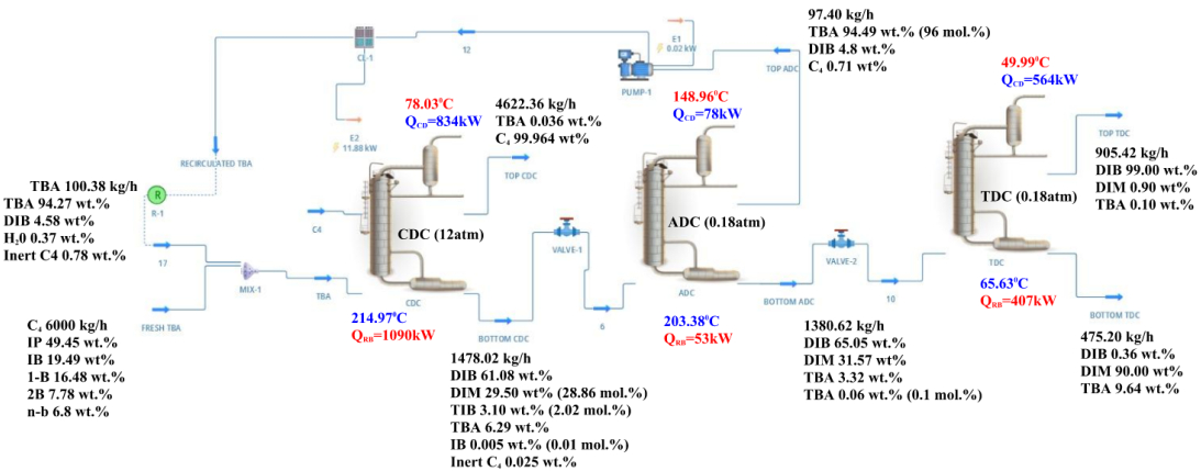
This study aimed to develop an artificial neural network (ANN) capable of predicting the molar concentration of diisobutylene (DIB), 3, 4, 4-trimethyl-1-pentene (DIM), and tert-butyl alcohol (TBA) in the distillate and residue streams within three specific columns: reactive (CDC), high pressure (ADC), and low pressure (TDC). The process simulation was conducted using DWSIM, an open-source platform. Following its validation, a sensitivity analysis was performed to identify the operational variables that influenced the molar fraction of DIB, DIM, and TBA in the outputs of the three columns. The input variables included the molar fraction of isobutylene (IB) and 2-butene (2-Bu) in the butane (C4) feed, the temperature of the C4 and TBA feeds, and the operating pressure of the CDC, ADC, and TDC columns. The network's design, training, validation, and testing were performed in MATLAB using the Neural FittinG app. The network structure was based on the Bayesian regularization (BR) algorithm, that consisted of 7 inputs and seven outputs with 30 neurons in the hidden layer. The designed, trained, and validated ANN demonstrated a high performance, with a mean squared error (MSE) of 0.0008 and a linear regression coefficient (R) of 0.9946. The statistical validation using an analysis of variance (ANOVA) (p-value > 0.05) supported the ANN's capability to reliably predict molar fractions. Future research will focus on the in-situ validation of the predictions and explore hybrid technologies for energy and environmental optimization in the process.

| [1] |
Honkela ML, Krause AOI (2003) Influence of polar components in the dimerization of isobutene. Catalysis Letters 87: 113–119. https://doi.org/10.1023/A:1023478703266 doi: 10.1023/A:1023478703266

|
| [2] |
Chen Z, Zhang Z, Zhou J, et al. (2021) Efficient synthesis of isobutylene dimerization by catalytic distillation with advanced heat-integrated technology. Ind Eng Chem Res 60: 6121–6136. https://doi.org/10.1021/acs.iecr.1c00945 doi: 10.1021/acs.iecr.1c00945
|
| [3] |
Liu J, Ding N, Ge Y, et al. (2019) Dimerization of Isobutene in C4 mixtures in the presence of ethanol over acid ion-exchange resin DH-2. Catal Letters 149: 1277–1285. https://doi.org/10.1007/s10562-019-02685-y doi: 10.1007/s10562-019-02685-y
|
| [4] |
Talwalkar S, Mankar S, Katariya A, et al. (2007) Selectivity engineering with reactive distillation for dimerization of C 4 Olefins: Experimental and theoretical studies. Ind Eng Chem Res 46: 3024–3034. https://doi.org/10.1021/ie060860+ doi: 10.1021/ie060860+
|
| [5] |
Kamath RS, Qi Z, Sundmacher K, et al. (2006) Process analysis for dimerization of isobutene by reactive distillation. Ind Eng Chem Res 45: 1575–1582. https://doi.org/10.1021/ie0506522 doi: 10.1021/ie0506522
|
| [6] |
Kamath RS, Qi Z, Sundmacher K, et al. (2006) Comparison of reactive distillation with process alternatives for the isobutene dimerization reaction. Ind Eng Chem Res 45: 2707–2714. https://doi.org/10.1021/ie051103z doi: 10.1021/ie051103z
|
| [7] |
Goortani BM, Gaurav A, Deshpande A, et al. (2015) Production of isooctane from isobutene: Energy integration and carbon dioxide abatement via catalytic distillation. Ind Eng Chem Res 54: 3570–3581. https://doi.org/10.1021/ie5032056 doi: 10.1021/ie5032056
|
| [8] | Chalakova M, Kaur R, Freund H, et al. (2007) Innovative reactive distillation process for the production of the MTBE substitute isooctane from isobutene. DGMK/SCI-Conference. Available from: https://www.osti.gov/etdeweb/servlets/purl/21074149 |
| [9] |
Zhang L, Sun X, Gao S (2022) Temperature prediction and analysis based on improved GA-BP neural network. AIMS Environ Sci 9: 735–753. https://doi.org/10.3934/environsci.2022042 doi: 10.3934/environsci.2022042
|
| [10] |
Nualtong K, Chinram R, Khwanmuang P, et al. (2021) An efficiency dynamic seasonal regression forecasting technique for high variation of water level in yom river basin of thailand. AIMS Environ Sci 8: 283–303. https://doi.org/10.3934/environsci.2021019 doi: 10.3934/environsci.2021019
|
| [11] |
Suphawan K, Chaisee K (2021) Gaussian process regression for predicting water quality index: A case study on ping river basin, thailand. AIMS Environ Sci 8: 268–282. https://doi.org/10.3934/environsci.2021018 doi: 10.3934/environsci.2021018
|
| [12] |
Zhang Z, Zhao J (2017) A deep belief network based fault diagnosis model for complex chemical processes. Comput Chem Eng 107: 395–407. https://doi.org/10.1016/j.compchemeng.2017.02.041 doi: 10.1016/j.compchemeng.2017.02.041
|
| [13] |
Chouai A, Laugier S, Richon D (2002) Modeling of thermodynamic properties using neural networks: Application to refrigerants. Fluid Phase Equilib 199: 53–62. https://doi.org/10.1016/S0378-3812(01)00801-9 doi: 10.1016/S0378-3812(01)00801-9
|
| [14] |
Manssouri I, Boudebbouz B, Boudad B (2021) Using artificial neural networks of the type extreme learning machine for the modelling and prediction of the temperature in the head the column. Case of a C6H11-CH3distillation column. Materials Today Proceedings 45: 7444–7449. https://doi.org/10.1016/j.matpr.2021.01.920 doi: 10.1016/j.matpr.2021.01.920
|
| [15] |
Alhajree I, Zahedi G, Manan ZA, et al. (2011) Modeling and optimization of an industrial hydrocracker plant. J Pet Sci Eng 78: 627–636. https://doi.org/10.1016/j.petrol.2011.07.019 doi: 10.1016/j.petrol.2011.07.019
|
| [16] | DWSIM (2020) DWSIM – The Open Source Chemical Process Simulator. Available from: https://dwsim.org |
| [17] |
Chuquin-Vasco D, Parra F, Chuquin-Vasco N, et al. (2021) Prediction of methanol production in a carbon dioxide hydrogenation plant using neural networks. Energies 14: 1–18. https://doi.org/10.3390/en14133965 doi: 10.3390/en14133965
|
| [18] | Dimian AC, Bildea CS, Kiss AA (2014) Introduction in process simulation, In Dimian. Integrated Design and Simulation of Chemical Processes 2 Eds., Amsterdam: Elsevier, 35–71. https://doi.org/10.1016/B978-0-444-62700-1.00002-4 |
| [19] | Kiss A (2013) Advanced distillation technologies - Design, control and applications. 1 Eds., Noida, India: Wiley. https://doi.org/10.1002/9781118543702 |
| [20] |
Soave G, Gamba S, Pellegrini L (2010) SRK equation of state: predicting binary interaction parameters of hydrocarbons and related compounds. Fluid Phase 299: 285–293. https://doi.org/10.1016/j.fluid.2010.09.012 doi: 10.1016/j.fluid.2010.09.012
|
| [21] |
Feng Z, Shen W, Rangaiah GP, et al. (2020) Design and control of vapor recompression assisted extractive distillation for separating n-hexane and ethyl acetate. Sep Purif Technol 240: 116655. https://doi.org/10.1016/j.seppur.2020.116655 doi: 10.1016/j.seppur.2020.116655
|
| [22] |
Singh V, Gupta I, Gupta HO (2005) ANN based estimator for distillation - Inferential control. Chem Eng Proces 44: 785–795. https://doi.org/10.1016/j.cep.2004.08.010 doi: 10.1016/j.cep.2004.08.010
|
| [23] | Pedregosa F, Varaquaux G, Gramfort A, et al. (2011) Scikit-learn: machine learning in Python. J Mach Lear Res. Available from: https://www.jmlr.org/papers/volume12/pedregosa11a/pedregosa11a.pdf |
| [24] |
Bloice M, Holzinger A (2016) A tutorial on machine learning and data science tools with python. Lect Not Comp Sci 9605: 435–480. https://doi.org/10.1007/978-3-319-50478-0_22 doi: 10.1007/978-3-319-50478-0_22
|
| [25] |
Chen Y, Song L, Liu Y, et al. (2020) A review of the artificial neural network models for water quality prediction. Appl Sci 10: 5776. https://doi.org/10.3390/app10175776 doi: 10.3390/app10175776
|
| [26] |
Zhang L, Sun X, Gao S (2022) Temperature prediction and analysis based on improved GA-BP neural network. AIMS Environ Sci 9: 735–753. https://doi.org/10.3934/environsci.2022042 doi: 10.3934/environsci.2022042
|
| [27] |
Wang L, Wu B, Zhu Q, et al. (2020) Forecasting Monthly Tourism Demand Using Enhanced Backpropagation Neural Network. Neural Process Lett 52: 2607–2636. https://doi.org/10.1007/s11063-020-10363-z doi: 10.1007/s11063-020-10363-z
|
| [28] |
Suphawan K, Chaisee K (2021) Gaussian process regression for predicting water quality index: A case study on ping river basin, thailand. AIMS Environ Sci 8: 268–282. https://doi.org/10.3934/environsci.2021018 doi: 10.3934/environsci.2021018
|
| [29] |
Chen Z, Zhang Z, Zhou J, et al. (2021) Efficient synthesis of isobutylene dimerization by catalytic distillation with advanced heat-integrated technology. Ind Eng Chem Res 60: 6121–6136. https://doi.org/10.1021/acs.iecr.1c00945 doi: 10.1021/acs.iecr.1c00945
|
| [30] |
Kayri M (2016) Predictive abilities of Bayesian regularization and levenberg-marquardt algorithms in artificial neural networks: A comparative empirical study on social data. Math Comp Appl 21: 20. https://doi.org/10.3390/mca21020020 doi: 10.3390/mca21020020
|
| [31] | Bharati S, Rahman M, Podder P, et al. (2019) Comparative Performance Analysis of Neural Network Base Training Algorithm and Neuro-Fuzzy System with SOM for the Purpose of Prediction of the Features of Superconductors. In: Abraham, A., Siarry, P., Ma, K., Kaklauskas, A. (eds) Intelligent Systems Design and Applications. ISDA 2019. Advances in Intelligent Systems and Computing 1181. https://doi.org/10.1007/978-3-030-49342-4_7 |
| [32] |
Saini LM (2008) Peak load forecasting using Bayesian regularization, Resilient and adaptive backpropagation learning based artificial neural networks. Elec Pow Syst Res 78: 1302–1310. https://doi.org/10.1016/j.epsr.2007.11.003 doi: 10.1016/j.epsr.2007.11.003
|
| [33] |
Wang L, Wu B, Zhu Q, et al. (2020) Forecasting Monthly Tourism Demand Using Enhanced Backpropagation Neural Network. Neural Process Lett 52: 2607–2636. https://doi.org/10.1007/s11063-020-10363-z doi: 10.1007/s11063-020-10363-z
|
| [34] |
Zeng YR, Zeng Y, Choi B, et al. (2017) Multifactor-influenced energy consumption forecasting using enhanced back-propagation neural network. Energy 127: 381–396. https://doi.org/10.1016/j.energy.2017.03.094 doi: 10.1016/j.energy.2017.03.094
|
| [35] |
Suliman A, Omarov B (2018) Applying Bayesian Regularization for Acceleration of Levenberg Marquardt based Neural Network Training. Int J Inte Mult Art Inte 5: 68. https://doi.org/10.9781/ijimai.2018.04.004 doi: 10.9781/ijimai.2018.04.004
|
| [36] |
Garoosiha H, Ahmadi J, Bayat H (2019) The assessment of Levenberg–Marquardt and Bayesian Framework training algorithm for prediction of concrete shrinkage by the artificial neural network. Cogent Eng 6: 1609179 https://doi.org/10.1080/23311916.2019.1609179 doi: 10.1080/23311916.2019.1609179
|
| [37] |
Abiodun O, Jantan A, Omolara A, et al. (2018) State of the art in artificial neural network applications: A survey. Heliyon 4: E00938. https://doi.org/10.1016/j.heliyon.2018.e00938 doi: 10.1016/j.heliyon.2018.e00938
|


Figures(14) / Tables(11)

Daniel Chuquin-Vasco, Geancarlo Torres-Yanacallo, Cristina Calderón-Tapia, Juan Chuquin-Vasco, Nelson Chuquin-Vasco, Ramiro Cepeda-Godoy. ANN for the prediction of isobutylene dimerization through catalytic distillation for a preliminary energy and environmental evaluation[J]. AIMS Environmental Science, 2024, 11(2): 157-183. doi: 10.3934/environsci.2024009


 DownLoad: