Characteristics of soil erosion in different land-use patterns under natural rainfall

Lei Wang; Huan Du; Jiajun Wu; Wei Gao; Linna Suo; Dan Wei; Liang Jin; Jianli Ding; Jianzhi Xie; Zhizhuang An; Lei Wang; Huan Du; Jiajun Wu; Wei Gao; Linna Suo; Dan Wei; Liang Jin; Jianli Ding; Jianzhi Xie; Zhizhuang An

doi:10.3934/environsci.2022021

AIMS Environmental Science

2022, Volume 9, Issue 3: 309-324. doi: 10.3934/environsci.2022021

Previous Article Next Article

Research article

Characteristics of soil erosion in different land-use patterns under natural rainfall

1.
Institute of Plant Nutrition, Resources and Environment, Beijing Academy of Agricultural and Forestry Sciences, Beijing 100097, China
2.
College of Resources and Environmental Sciences, Agricultural University of Hebei, Baoding, Hebei 071000, China
3.
Sichuan Water Conservancy College, Chengdu, Sichuan 610000, China
^† These two authors contributed equally.

Received: 28 March 2022 Revised: 14 June 2022 Accepted: 15 June 2022 Published: 21 June 2022

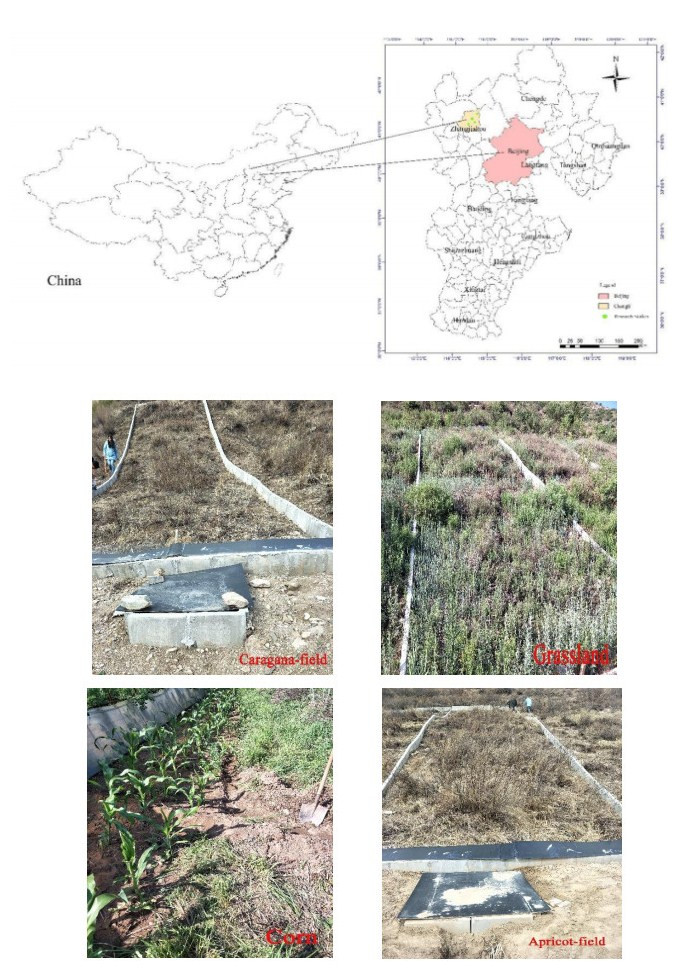
Land degradation due to soil erosion is a major problem in mountainous areas. It is crucially important to understand the law of soil erosion under different land-use patterns with rainfall variability. We studied Qingshuihe Watershed in the Chongli district of the Zhangjiakou area. Four runoff plots, including caragana, corn, apricot trees, and barren grassland, were designed on the typical slopes of Xigou and Donggou locations. The 270 natural rainfall events observed from 2014 to 2016 were used to form a rainfall gradient. The relationship between runoff and sediment yield was analyzed. Results showed that the monthly rainfall of the slope runoff plot in the Chongli mountain area presented the trend of concentrated rainfall in summer, mainly from June to September, accounting for 82.4% of the total rainfall in 2014–2016, which was far higher than that in other months. Starting from April to May every year, the rainfall increased with time, then from July to September, the rainfall decreased gradually, but it was still at the high level of the whole year. Among the four ecosystems, the caragana-field has the best effect on reducing the kinetic energy of rainfall and runoff, which can effectively reduce the runoff and sediment yield of the slope and reduce the intensity of soil erosion. In terms of the total amount of runoff and sediment, the runoff and sediment yield of the caragana-field reduced by 74%–87% and 64%–86% compared with that of the grassland. Comparing different land-use types, the caragana plantation would be conducive to conserving soil and water resources.
- Qingshuihe watershed,
- natural rainfall,
- characteristics of soil erosion
Citation: Lei Wang, Huan Du, Jiajun Wu, Wei Gao, Linna Suo, Dan Wei, Liang Jin, Jianli Ding, Jianzhi Xie, Zhizhuang An. Characteristics of soil erosion in different land-use patterns under natural rainfall[J]. AIMS Environmental Science, 2022, 9(3): 309-324. doi: 10.3934/environsci.2022021

Related Papers:

Abstract

Land degradation due to soil erosion is a major problem in mountainous areas. It is crucially important to understand the law of soil erosion under different land-use patterns with rainfall variability. We studied Qingshuihe Watershed in the Chongli district of the Zhangjiakou area. Four runoff plots, including caragana, corn, apricot trees, and barren grassland, were designed on the typical slopes of Xigou and Donggou locations. The 270 natural rainfall events observed from 2014 to 2016 were used to form a rainfall gradient. The relationship between runoff and sediment yield was analyzed. Results showed that the monthly rainfall of the slope runoff plot in the Chongli mountain area presented the trend of concentrated rainfall in summer, mainly from June to September, accounting for 82.4% of the total rainfall in 2014–2016, which was far higher than that in other months. Starting from April to May every year, the rainfall increased with time, then from July to September, the rainfall decreased gradually, but it was still at the high level of the whole year. Among the four ecosystems, the caragana-field has the best effect on reducing the kinetic energy of rainfall and runoff, which can effectively reduce the runoff and sediment yield of the slope and reduce the intensity of soil erosion. In terms of the total amount of runoff and sediment, the runoff and sediment yield of the caragana-field reduced by 74%–87% and 64%–86% compared with that of the grassland. Comparing different land-use types, the caragana plantation would be conducive to conserving soil and water resources.

References

[1]	Bouguerra S, Jebari S, Tarhouni J (2020) Spatiotemporal analysis of landscape patterns and its effect on soil loss in the Rmel river basin, Tunisia. Soil and Water Research 16: 39–49. http://doi.org/10.17221/84/2019-SWR doi: 10.17221/84/2019-SWR
[2]	Flores BM, Staal A, Jakovac CC, et al. (2020) Correction to: Soil erosion as a resilience drain in disturbed tropical forests. Plant and Soil 450: 27–28. http://doi.org/10.1007/s11104-019-04286-5 doi: 10.1007/s11104-019-04286-5
[3]	Thapa P (2020) Spatial estimation of soil erosion using RUSLE modeling: a case study of Dolakha district, Nepal. Environmental Systems Research 9: 1–10. http://doi.org/10.1186/s40068-020-00177-2 doi: 10.1186/s40068-020-00177-2
[4]	Keesstra S, Mol G, De Leeuw J, et al. (2018) Soil-related sustainable development goals: Four concepts to make land degradation neutrality and restoration work. Land 7: 133. http://doi.org/10.3390/land7040133 doi: 10.3390/land7040133
[5]	Keesstra S, Sannigrahi S, López-Vicente M, et al. (2021) The role of soils in regulation and provision of blue and green water. Philosophical Transactions of the Royal Society B 376: 20200175. http://doi.org/10.1098/RSTB.2020.0175 doi: 10.1098/RSTB.2020.0175
[6]	Mohamadi MA, Kavian A (2015) Effects of rainfall patterns on runoff and soil erosion in field plots. International soil and water conservation research 3: 273–281. http://doi.org/10.1016/j.iswcr.2015.10.001 doi: 10.1016/j.iswcr.2015.10.001
[7]	Zhao B, Zhang L, Xia Z, et al. (2019) Effects of rainfall intensity and vegetation cover on erosion characteristics of a soil containing rock fragments slope. Advances in civil engineering 2019. https://doi.org/10.1155/2019/7043428 doi: 10.1155/2019/7043428
[8]	Sartori M, Philippidis G, Ferrari E, et al. (2019) A linkage between the biophysical and the economic: Assessing the global market impacts of soil erosion. Land use policy 86: 299–312. https://doi.org/10.1016/j.landusepol.2019.05.014 doi: 10.1016/j.landusepol.2019.05.014
[9]	Montanarella L, Badraoui M, Chude V, et al. (2015) Status of the world's soil resources: main report. Embrapa Solos-Livro científico (ALICE).
[10]	Cai M, An C, Guy C, et al. (2020) Assessment of soil and water conservation practices in the loess hilly region using a coupled rainfall-runoff-erosion model. Sustainability 12: 934. https://doi.org/10.3390/su12030934 doi: 10.3390/su12030934
[11]	Visconti D, Fiorentino N, Cozzolino E, et al. (2020) Use of giant reed (Arundo donax L.) to control soil erosion and improve soil quality in a marginal degraded area. Italian Journal of Agronomy 15: 332–338. https://doi.org/10.4081/ija.2020.1764 doi: 10.4081/ija.2020.1764
[12]	Shi P, Schulin R (2018) Erosion-induced losses of carbon, nitrogen, phosphorus and heavy metals from agricultural soils of contrasting organic matter management. Science of the Total Environment 618: 210–218. https://doi.org/10.1016/j.scitotenv.2017.11.060 doi: 10.1016/j.scitotenv.2017.11.060
[13]	Fiener P, Auerswald K, Van Oost K (2011) Spatio-temporal patterns in land use and management affecting surface runoff response of agricultural catchments—A review. Earth-Science Reviews 106: 92–104. https://doi.org/10.1016/j.earscirev.2011.01.004 doi: 10.1016/j.earscirev.2011.01.004
[14]	Worrall F, Burt TP, Howden N J (2016) The fluvial flux of particulate organic matter from the UK: the emission factor of soil erosion. Earth Surface Processes and Landforms 41: 61–71. https://doi.org/10.1002/esp.3795 doi: 10.1002/esp.3795
[15]	Berhe AA, Harden JW, Torn MS, et al. (2008) Linking soil organic matter dynamics and erosion‐induced terrestrial carbon sequestration at different landform positions. Journal of Geophysical Research: Biogeosciences 113. https://doi.org/10.1029/2008JG000751 doi: 10.1029/2008JG000751
[16]	She D, Liu Y, Shao MA, et al. (2012) Simulated effects and adaptive evaluation of different canopies rainfall interception models in Loess Plateau. Transactions of the Chinese Society of Agricultural Engineering 28: 115–120.
[17]	Guo Z, Shao M (2013) Impact of afforestation density on soil and water conservation of the semiarid Loess Plateau, China. Journal of Soil and water conservation 68: 401–410. https://doi.org/10.2489/jswc.68.5.401 doi: 10.2489/jswc.68.5.401
[18]	Wang L, Xie J, Luo Z, et al. (2021). Forage yield, water use efficiency, and soil fertility response to alfalfa growing age in the semiarid Loess Plateau of China. Agricultural Water Management 243: 106415. https://doi.org/10.1016/j.agwat.2020.106415 doi: 10.1016/j.agwat.2020.106415
[19]	Zhao H, He H, Wang J, et al. (2018) Vegetation restoration and its environmental effects on the Loess Plateau. Sustainability 10: 4676. https://doi.org/10.3390/su10124676 doi: 10.3390/su10124676
[20]	Pan T, Zuo L, Zhang Z, et al. (2020) Impact of land use change on water conservation: a case study of Zhangjiakou in Yongding River. Sustainability 13: 22. https://doi.org/10.3390/SU13010022 doi: 10.3390/SU13010022
[21]	Chu X, Deng X, Jin G, et al. (2017) Ecological security assessment based on ecological footprint approach in Beijing-Tianjin-Hebei region, China. Physics and Chemistry of the Earth 101: 43–51. https://doi.org/10.1016/j.pce.2017.05.001 doi: 10.1016/j.pce.2017.05.001
[22]	Li M, Yao W, Shen Z, et al. (2016) Erosion rates of different land uses and sediment sources in a watershed using the137Cs tracing method: Field studies in the Loess Plateau of China. Environmental Earth Sciences 75: 1–10. https://doi.org/10.1007/s12665-015-5225-6 doi: 10.1007/s12665-015-5225-6
[23]	Cerdà A, Novara A, Moradi E. (2021) Long-term non-sustainable soil erosion rates and soil compaction in drip-irrigated citrus plantation in Eastern Iberian Peninsula. Science of the Total Environment 787: 147549. https://doi.org/10.1016/J.SCITOTENV.2021.147549. doi: 10.1016/J.SCITOTENV.2021.147549
[24]	Rodrigo Comino J, Keesstra SD, Cerdà A (2018) Connectivity assessment in Mediterranean vineyards using improved stock unearthing method, LiDAR and soil erosion field surveys. Earth Surface Processes and Landforms 43: 2193–2206. https://doi.org/10.1002/esp.4385 doi: 10.1002/esp.4385
[25]	Keesstra SD, Davis J, Masselink RH, et al. (2019) Coupling hysteresis analysis with sediment and hydrological connectivity in three agricultural catchments in Navarre, Spain. Journal of Soils and Sediments 19: 1598–1612. https://doi.org/10.1007/s11368-018-02223-0 doi: 10.1007/s11368-018-02223-0
[26]	Cerdà Artemi TE, Daliakopoulos IN (2021) Weed cover controls soil and water losses in rainfed olive groves in Sierra de Enguera, eastern Iberian Peninsula. Journal of Environmental Management 290: 112516. https://doi.org/10.1016/J.JENVMAN.2021.112516. doi: 10.1016/J.JENVMAN.2021.112516
[27]	Wang X, He K, Dong Z (2019) Effects of climate change and human activities on runoff in the Beichuan River Basin in the northeastern Tibetan Plateau, China. Catena 176: 81–93. https://doi.org/10.1016/j.catena.2019.01.001 doi: 10.1016/j.catena.2019.01.001
[28]	Fang NF, Wang L, Shi ZH (2017) Runoff and soil erosion of field plots in a subtropical mountainous region of China. Journal of Hydrology 552: 387–395. https://doi.org/10.1016/j.jhydrol.2017.06.048 doi: 10.1016/j.jhydrol.2017.06.048
[29]	Chen H, Zhang X, Abla M, et al. (2018) Effects of vegetation and rainfall types on surface runoff and soil erosion on steep slopes on the Loess Plateau, China. Catena 170: 141–149. https://doi.org/10.1016/j.catena.2018.06.006 doi: 10.1016/j.catena.2018.06.006
[30]	Deng L, Kim DG, Li M, et al. (2019) Land-use changes driven by 'Grain for Green'program reduced carbon loss induced by soil erosion on the Loess Plateau of China. Global and planetary change 177: 101–115. https://doi.org/10.1016/j.gloplacha.2019.03.017 doi: 10.1016/j.gloplacha.2019.03.017
[31]	Bogale A, Aynalem D, Adem A, et al. (2020) Spatial and temporal variability of soil loss in gully erosion in upper Blue Nile basin, Ethiopia. Applied Water Science 10: 1–8. https://doi.org/10.1007/s13201-020-01193-4. doi: 10.1007/s13201-020-01193-4
[32]	Sun C, Hou H, Chen W (2021) Effects of vegetation cover and slope on soil erosion in the Eastern Chinese Loess Plateau under different rainfall regimes. PeerJ 9: e11226. https://doi.org/10.7717/PEERJ.11226. doi: 10.7717/PEERJ.11226
[33]	de Almeida WS, Seitz S, de Oliveira LFC, et al. (2021). Duration and intensity of rainfall events with the same erosivity change sediment yield and runoff rates. International Soil and Water Conservation Research 9: 69–75. https://doi.org/10.1016/j.iswcr.2020.10.004. doi: 10.1016/j.iswcr.2020.10.004
[34]	Zeng Q, Lal R, Chen Y, et al. (2017) Soil, leaf and root ecological stoichiometry of Caragana korshinskii on the Loess Plateau of China in relation to plantation age. PLoS One 12: e0168890. https://doi.org/10.1371/journal.pone.0168890. doi: 10.1371/journal.pone.0168890
[35]	Liang Y, Jiao JY, Tang BZ, et al. (2020) Response of runoff and soil erosion to erosive rainstorm events and vegetation restoration on abandoned slope farmland in the Loess Plateau region, China. Journal of Hydrology 584: 124694. https://doi.org/10.1016/j.jhydrol.2020.124694. doi: 10.1016/j.jhydrol.2020.124694
[36]	Chen X, Zhang X, Zhang Y, et al. (2009) Carbon sequestration potential of the stands under the Grain for Green Program in Yunnan Province, China. Forest Ecology and Management 258: 199–206. https://doi.org/10.1016/j.foreco.2008.07.010 doi: 10.1016/j.foreco.2008.07.010
[37]	Wolf B, Kiese R, Chen W, et al. (2012) Modeling N2O emissions from steppe in Inner Mongolia, China, with consideration of spring thaw and grazing intensity. Plant and soil 350: 297–310. https://doi.org/10.1007/s11104-011-0908-6 doi: 10.1007/s11104-011-0908-6
[38]	Deng L, Liu GB, Shangguan ZP (2014) Land‐use conversion and changing soil carbon stocks in C hina's 'Grain‐for‐Green'Program: a synthesis. Global Change Biology 20: 3544–3556. https://doi.org/10.1111/gcb.12508 doi: 10.1111/gcb.12508
[39]	Wang D, Liu Y, Shang ZH, et al. (2015). Effects of grassland conversion from cropland on soil respiration on the semi‐arid loess plateau, China. CLEAN–Soil, Air, Water 43: 1052–1057. https://doi.org/10.1002/clen.201300971 doi: 10.1002/clen.201300971
[40]	Cheng J, Cheng J, Hu T, et al. (2012) Dynamic changes of Stipa bungeana steppe species diversity as better indicators for soil quality and sustainable utilization mode in Yunwu Mountain Nature Reserve, Ningxia, China. CLEAN–Soil, Air, Water 40: 127–133. https://doi.org/10.1002/clen.201000438 doi: 10.1002/clen.201000438
[41]	Tang L, Zhang Z, Wang X, et al. (2010) Effects of precipitation and land use/cover variability on erosion and sediment yield in Qingshuihe Watershed on the Loess Plateau. China. J Nat Resour 8.
[42]	Zhu KB, Li ZH, Yang SP (2014) Features and Assessment of Ecological Restoration Models of Qingshuihe Watershed in Rainstorm Center Area. Bulletin of Soil & Water Conservation 4: 193–197.

Reader Comments

Your name:*

Email:*
© 2022 the Author(s), licensee AIMS Press. This is an open access article distributed under the terms of the Creative Commons Attribution License (http://creativecommons.org/licenses/by/4.0)