Universal design as resilient urban space plan strategy. New scenarios for environmental resources' sustainable management

Sonia Prestamburgo; Filippo Sgroi; Adriano Venudo; Carlo Zanin; Sonia Prestamburgo; Filippo Sgroi; Adriano Venudo; Carlo Zanin

doi:10.3934/environsci.2021021

AIMS Environmental Science

2021, Volume 8, Issue 4: 321-340. doi: 10.3934/environsci.2021021

Previous Article Next Article

Research article

Universal design as resilient urban space plan strategy. New scenarios for environmental resources' sustainable management

1.
Department of Engineering and Architecture, University of Trieste, Trieste 34127, Italy
2.
Department of Agricultural and Forestry Sciences, University of Palermo, Palermo 90128, Italy
3.
Department of Engineering and Architecture, University of Trieste, Trieste 34127, Italy
4.
Community Welfare Area, Friuli Venezia Giulia Region, Palmanova, Udine 33100, Italy

Received: 03 June 2021 Accepted: 04 July 2021 Published: 15 July 2021

Nowadays, urban framework, stressed by the growing anthropic pressure and its constantly evolving use requests is split by uneven structures, contexts, users and patchy needs, which come out to be inefficient and ineffective in access and management. This fact is directly connected both with morph-functional structure of urban texture and its continuous changing trends. The most important consequences of this situation are some negative effects that produce entropy, mistaken anthropic space uses, ecological networks decrease and most of all a substantial urban life quality reduction connected with mobility problems and non-resilient spaces' use at the different plan scales. These elements make it necessary to restart thinking about environmental resources' sustainable use and management. Universal design comes out to be a useful tool related to urban space planning strategies in terms of resilient choices and actions. Design for all plan approach also represents a good solution for matching people needs to urban environmental quality improvement.

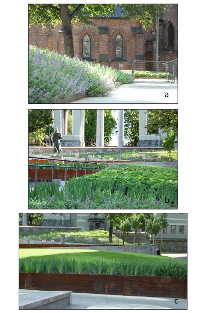
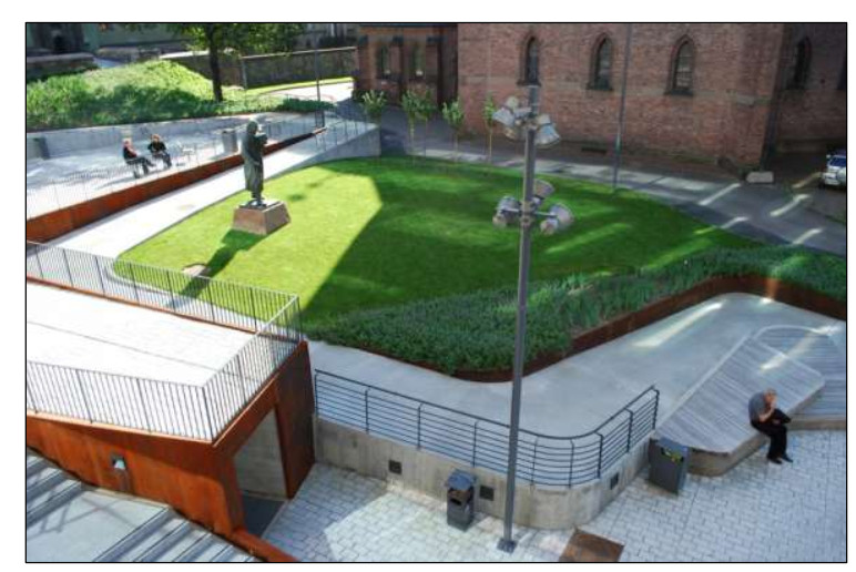
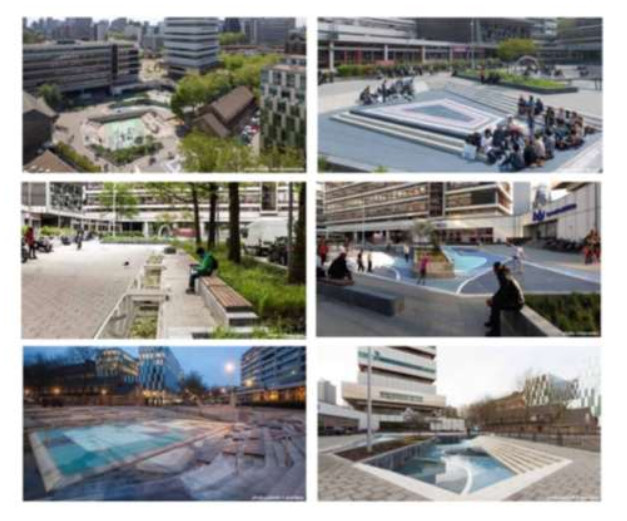
This idea is supported by the experience of a certain case study, that considers universal design application positive effects on open public space plan strategy in Oslo, together with an example of an active use of water to plan a sustainable public space in Rotterdam.
- universal design,
- urban context,
- plan strategy,
- resilience,
- environmental resources
Citation: Sonia Prestamburgo, Filippo Sgroi, Adriano Venudo, Carlo Zanin. Universal design as resilient urban space plan strategy. New scenarios for environmental resources' sustainable management[J]. AIMS Environmental Science, 2021, 8(4): 321-340. doi: 10.3934/environsci.2021021

Related Papers:

Abstract

Nowadays, urban framework, stressed by the growing anthropic pressure and its constantly evolving use requests is split by uneven structures, contexts, users and patchy needs, which come out to be inefficient and ineffective in access and management. This fact is directly connected both with morph-functional structure of urban texture and its continuous changing trends. The most important consequences of this situation are some negative effects that produce entropy, mistaken anthropic space uses, ecological networks decrease and most of all a substantial urban life quality reduction connected with mobility problems and non-resilient spaces' use at the different plan scales. These elements make it necessary to restart thinking about environmental resources' sustainable use and management. Universal design comes out to be a useful tool related to urban space planning strategies in terms of resilient choices and actions. Design for all plan approach also represents a good solution for matching people needs to urban environmental quality improvement.

This idea is supported by the experience of a certain case study, that considers universal design application positive effects on open public space plan strategy in Oslo, together with an example of an active use of water to plan a sustainable public space in Rotterdam.

References

[1]	UN Convention on the Rights of Persons with Disabilities (UNCRPD), Final Report. December 2006.
[2]	Iwarsson S, Stahl A, (2003) Accessibility, usability and universal design. Positioning and definition of concepts describing person-environment relationships. Disability and Rehabilitation 25 (2): 57-66.
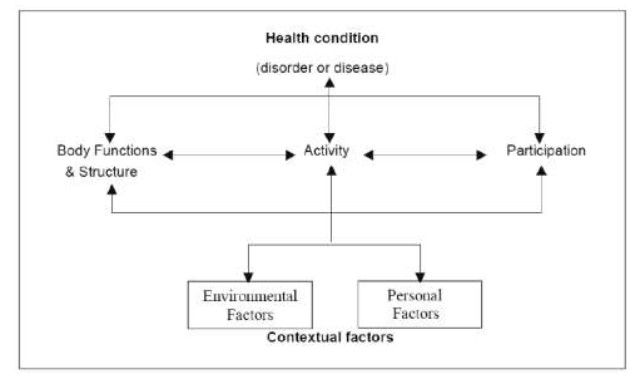
[3]	International Classification of Functioning, Disability and Health (ICF), WHO, 2001) Available from: https://www.who.int/standards/classifications/international-classification-of-functioning-disability-and-health
[4]	Bergamo M, (2002) Architettura, linguaggio, contesto, Libreria EditriceCarfoscarina, Venezia (in Italian).
[5]	Heidegger M, (2000) L'origine dell'opera d'arte. Testo tedesco a fronte, Zaccaria G., De Gennaro I, (a cura di), Christian Marinotti Edizioni, Milano (in Italian).
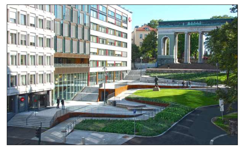
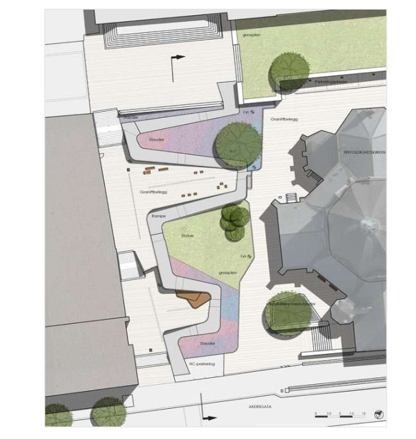
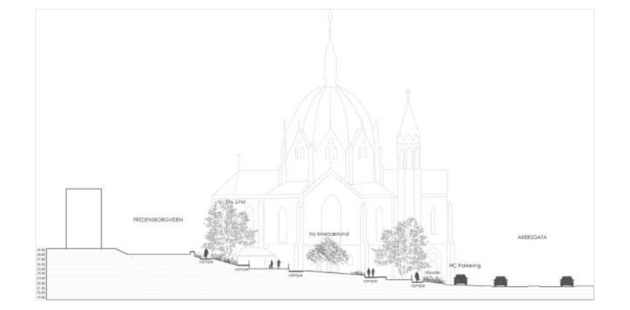
[6]	Østengen & Bergo AS, landscape architects; Available from: https://ostengen-bergo.no/prosjekt/schandorffs-plass-2/.
[7]	Le Corbusier-Saugnier, (1923) Vers une Architecture, Crès et Cie, Éditions Crès. Collection de "L'Esprit Nouveau". Fondation Le Corbusier, Paris.
[8]	Careri F, (2006) Walkscapes. Camminare come pratica estetica. Piccola Biblioteca Einaudi, Giulio Einaudi Editore, Torino (in Italian).
[9]	Benevolo L, (1991) La cattura dell'infinito, Collana Quadrante Laterza, Editori Laterza, Bari (in Italian).
[10]	Available from: DE URBANISTEN Project Architect, 2012.
[11]	Boffi M, (2012) Metodo e misurazione dell'accessibilità urbana, in Castrignanò M., Colleoni M., Pronello C. (a cura di), Muoversi in città. Accessibilità e mobilità nella metropoli contemporanea, Franco Angeli Edizioni, Milano (in Italian).
[12]	De Rubertis R. Il disagio dell'architettura. 1994.
[13]	Costa M, (2013) Psicologia ambientale e architettonica. Come l'ambiente e l'architettura influenzano la mente e il comportamento, Collana Psicologia, Franco Angeli Edizioni, Milano (in Italian).
[14]	Basilico G, Boeri S, (1997) Sezioni del paesaggio italiano. Art & Editore, Udine (in Italian).
[15]	Bauman Z (2008) Modus vivendi. Inferno e utopia nel mondo liquido, Collana Economica Laterza, Editori Laterza, Bari (in Italian).
[16]	Gabrielli A (2015) Grande Dizionario Hoepli Italiano, Hoepli Edizioni Milano (in Italian).
[17]	De Simone I, (2015) Progettare l'accessibilità urbana: modelli e strategie per la trasformazione della città contemporanea. Tesi di dottorato. Scuola di Dottorato in Scienze dell'Architettura, Dottorato di Ricerca in Architettura – Teorie e Progetto, XXVII ciclo. Sapienza, Università di Roma. Coll. 17/C: 28 (in Italian).
[18]	Lynch K (1990) Progettare la città. La qualità della forma urbana, EtasLibri, Milano (in Italian).
[19]	Garofolo I, Marchigiani E (2019) Accessibility and the City. A Trieste, dispositivi e pratiche progettuali per attenuare le vulnerabilità sociali. Atti XXI Conferenza nazionale SIU. Confini, Movimenti, Luoghi. Politiche e Progetti per Città e territori in Transizione, Firenze, 6-8 giugno 2018. Planum Publisher, Roma-Milano (in Italian).
[20]	Lynch, K (1960) The Image of the City. Publication of the Joint Center for Urban Studies, Cambridge Mass. MIT Press, USA.

Reader Comments

Your name:*

Email:*
© 2021 the Author(s), licensee AIMS Press. This is an open access article distributed under the terms of the Creative Commons Attribution License (http://creativecommons.org/licenses/by/4.0)