Solar radiation forecasting based on ANN, SVM and a novel hybrid FFA-ANN model: A case study of six cities south of Algeria

Halima Djeldjli; Djelloul Benatiallah; Camel Tanougast; Ali Benatiallah; Halima Djeldjli; Djelloul Benatiallah; Camel Tanougast; Ali Benatiallah

doi:10.3934/energy.2024004

AIMS Energy

2024, Volume 12, Issue 1: 62-83. doi: 10.3934/energy.2024004

Previous Article Next Article

Research article

Solar radiation forecasting based on ANN, SVM and a novel hybrid FFA-ANN model: A case study of six cities south of Algeria

1.
Material Sciences Department, Faculty of Material Sciences, Mathematics and Computer Science Laboratory of Sustainable Development and Computer Science (LSDCS), University Ahmed Draia, Adrar, 01000, Algeria
2.
Laboratory of Systems Design, Optimization and Modeling (LCOMS), University of Lorraine, Metz 57070, France
3.
Laboratory of Energy Environment and Information System (LEEIS), University Ahmed Draia, Adrar, 01000, Algeria

Received: 30 October 2023 Revised: 06 December 2023 Accepted: 11 December 2023 Published: 27 December 2023

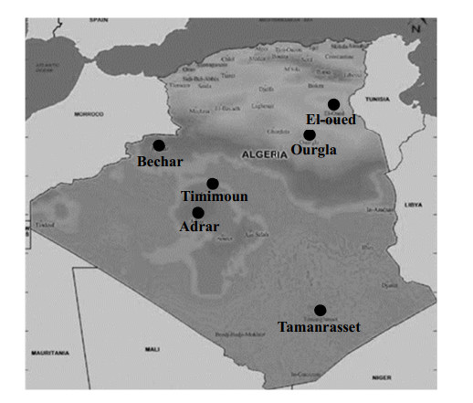
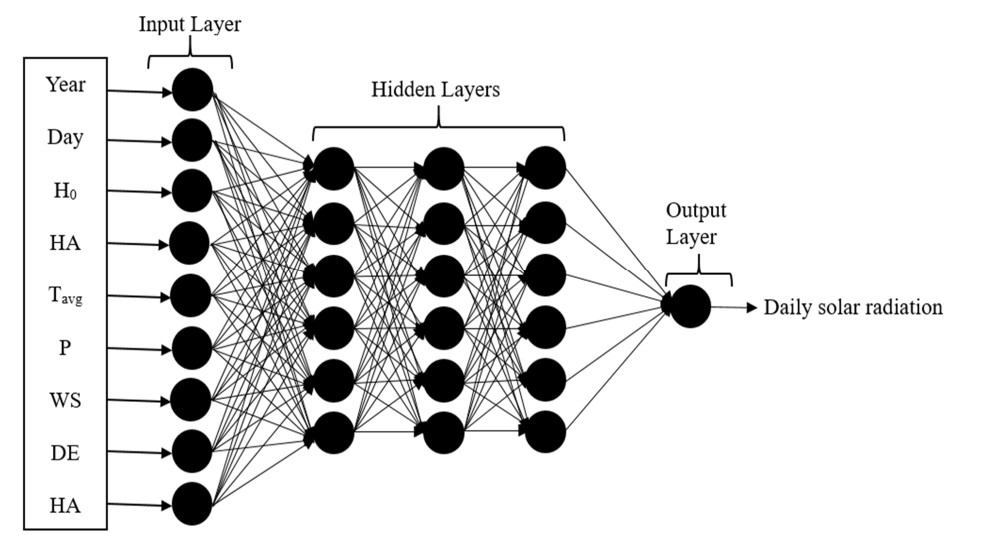
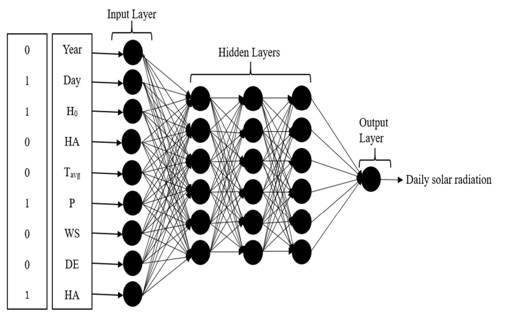
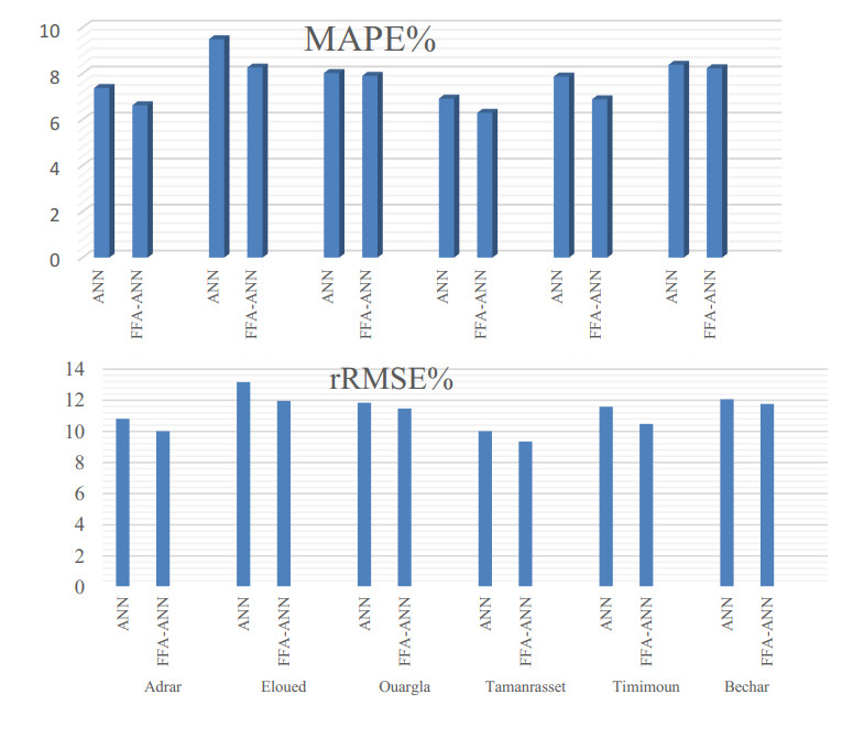
This study was conducted for six cities in southern Algeria, where the accuracy of three models—support vector machines (SVM), artificial neural networks (ANN) and a novel hybrid firefly algorithm-based model (FFA-ANN)—were investigated when estimating global solar irradiation throughout an eleven-year period, utilizing nine input parameters as input data. The goal of our novel suggested a hybrid FFA-ANN model, where we relied on the optimization Firefly algorithm to enhance the ANN model created. Despite the fact that the ANN and SVM models produced promising results, our suggested FFA-ANN hybrid model outperformed the stand-alone ANN-based model using three statistical factors—correlation coefficient, relative root mean squared error and mean absolute percent error—with the best values of (R = 0.9321, rRMSE = 9.35% and MAPE = 6.29%). The findings demonstrated that FFA-ANN was preferable to the optimized SVM and ANN models when forecasting daily global solar irradiation in all zones. Furthermore, after comparing the combinations, the study's findings showed that the ANN model depended on: Extraterrestrial solar irradiation (H₀), declination and average temperature (T_avg) together with relative humidity (RH) as inputs in order to estimate daily sun radiation. Thus, the findings of this study suggest that in regions with dry climates and other places with comparable climates, the created model may be used to estimate daily global solar radiation whenever data is accessible.
- hybrid model,
- artificial neural network (ANN),
- firefly algorithm (FFA),
- solar radiation,
- optimization,
- energy systems,
- support vector machine (SVM)
Citation: Halima Djeldjli, Djelloul Benatiallah, Camel Tanougast, Ali Benatiallah. Solar radiation forecasting based on ANN, SVM and a novel hybrid FFA-ANN model: A case study of six cities south of Algeria[J]. AIMS Energy, 2024, 12(1): 62-83. doi: 10.3934/energy.2024004

Related Papers:

Abstract

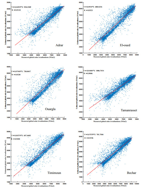
This study was conducted for six cities in southern Algeria, where the accuracy of three models—support vector machines (SVM), artificial neural networks (ANN) and a novel hybrid firefly algorithm-based model (FFA-ANN)—were investigated when estimating global solar irradiation throughout an eleven-year period, utilizing nine input parameters as input data. The goal of our novel suggested a hybrid FFA-ANN model, where we relied on the optimization Firefly algorithm to enhance the ANN model created. Despite the fact that the ANN and SVM models produced promising results, our suggested FFA-ANN hybrid model outperformed the stand-alone ANN-based model using three statistical factors—correlation coefficient, relative root mean squared error and mean absolute percent error—with the best values of (R = 0.9321, rRMSE = 9.35% and MAPE = 6.29%). The findings demonstrated that FFA-ANN was preferable to the optimized SVM and ANN models when forecasting daily global solar irradiation in all zones. Furthermore, after comparing the combinations, the study's findings showed that the ANN model depended on: Extraterrestrial solar irradiation (H₀), declination and average temperature (T_avg) together with relative humidity (RH) as inputs in order to estimate daily sun radiation. Thus, the findings of this study suggest that in regions with dry climates and other places with comparable climates, the created model may be used to estimate daily global solar radiation whenever data is accessible.

References

[1]	Kabouche N, Chellali F, Recioui A (2021) A review on solar radiation assessment and forecasting in Algeria: (Part 2; Solar radiation forecasting). Algerian J Sign Syst 6: 130–146. https://doi.org/10.51485/ajss.v6i3.141 doi: 10.51485/ajss.v6i3.141
[2]	Gairaa K, Khellaf A, Messlem Y, et al. (2016) Estimation of the daily global solar radiation based on Box–Jenkins and ANN models: A combined approach. Renewable Sustainable Energy Rev 57: 238–249. https://doi.org/10.1016/j.rser.2015.12.111 doi: 10.1016/j.rser.2015.12.111
[3]	Benatiallah D, Benatiallah A, Bouchouicha K, et al. (2020) Prediction of hourly solar radiation using artificial neural networks. Algerian J Env Sci Technol 6: 1236–1245. Available from: https://www.aljest.net/index.php/aljest/article/view/272.
[4]	Antonopoulos VZ, Papamichail DM, Aschonitis VG, et al. (2019) Solar radiation estimation methods using ANN and empirical models. Comp Electron Agric 160: 160–167. https://doi.org/10.1016/j.compag.2019.03.022 doi: 10.1016/j.compag.2019.03.022
[5]	Amiri B, Gómez-Orellana AM, Gutiérrez PA, et al. (2020) A novel approach for global solar irradiation forecasting on tilted plane using hybrid evolutionary neural networks. J Clean Produc 287: 125577. https://doi.org/10.1016/j.jclepro.2020.125577 doi: 10.1016/j.jclepro.2020.125577
[6]	Alsina EF, Bortolini M, Gamberi M, et al. (2016) Artificial neural network optimisation for monthly average daily global solar radiation prediction. Energy Conv Manag 120: 320–329. https://doi.org/10.1016/j.enconman.2016.04.101 doi: 10.1016/j.enconman.2016.04.101
[7]	Assas O, Bouzgou H, Fetah S, et al. (2014) Use of the artificial neural network and meteorological data for predicting daily global solar radiation in Djelfa, Algeria. 2014 Int Conf on Composite Materials Renewable Energy Applications (ICCMREA), Sousse, Tunisia, 1–5. https://doi.org/10.1109/ICCMREA.2014.6843807
[8]	Voyant C, Muselli M, Paoli C, et al. (2011) Optimization of an artificial neural network dedicated to the multivariate forecasting of daily global radiation. Energy 36: 348–359 https://doi.org/10.1016/j.energy.2010.10.032 doi: 10.1016/j.energy.2010.10.032
[9]	Hasni A, Sehli A, Draoui B, et al. (2012) Estimating global solar radiation using artificial neural network and climate data in the south-western region of Algeria. Energy Proc 18: 531–537. https://doi.org/10.1016/j.egypro.2012.05.064 doi: 10.1016/j.egypro.2012.05.064
[10]	Meenal R, Immanuel Selvakumar A (2018) Assessment of SVM, Empirical and ANN based solar radiation prediction models with most influencing input parameters. Renewable Energy 121: 324–343. https://doi.org/10.1016/j.renene.2017.12.005
[11]	Mohammadi K, Shamshirband S, Danesh AS, et al. (2020) Retracted article: Horizontal global solar radiation estimation using hybrid SVM-firefly and SVM-wavelet algorithms: A case study. Natural Hazards 102: 1613–1614. https://doi.org/10.1007/s11069-015-2047-5 doi: 10.1007/s11069-015-2047-5
[12]	Guermoui M, Rabehi A, Gairaa K, et al. (2018) Support vector regression methodology for estimating global solar radiation in Algeria. European Phys J Plus 133: 22. https://doi.org/10.1140/epjp/i2018-11845-y doi: 10.1140/epjp/i2018-11845-y
[13]	Guijo-Rubio D, Durán-Rosal AM, Gutiérrez PA, et al. (2020) Evolutionary artificial neural networks for accurate solar radiation prediction. Energy 210: 118374. https://doi.org/10.1016/j.energy.2020.118374 doi: 10.1016/j.energy.2020.118374
[14]	Belaid S, Mellit A (2016) Prediction of daily and mean monthly global solar radiation using support vector machine in an arid climate. Energy Conver Manage 118: 105–118. https://doi.org/10.1016/j.enconman.2016.03.082 doi: 10.1016/j.enconman.2016.03.082
[15]	Shamshirband S, Mohammadi K, Khorasanizadeh H, et al. (2016) Estimating the diffuse solar radiation using a coupled support vector machine-wavelet transform model. Renewable Sustainable Energy Rev 56: 428–435. https://doi.org/10.1016/j.rser.2015.11.055 doi: 10.1016/j.rser.2015.11.055
[16]	Bakhashwain JM (2016) Prediction of global solar radiation using support vector machines. Int J Green Energy 13: 1467–1472. https://doi.org/10.1080/15435075.2014.896256 doi: 10.1080/15435075.2014.896256
[17]	Baser F, Demirhan H (2017) A fuzzy regression with support vector machine approach to the estimation of horizontal global solar radiation. Energy 123: 229–240 https://doi.org/10.1016/j.energy.2017.02.008 doi: 10.1016/j.energy.2017.02.008
[18]	Queja VH, Almoroxa J, Arnaldob JA, et al. (2017) ANFIS, SVM and ANN soft-computing techniques to estimate daily global solar radiation in a warm sub-humid environment. J Atmos Sol-Terrestrial Physic 155: 62–70. https://doi.org/10.1016/j.jastp.2017.02.002 doi: 10.1016/j.jastp.2017.02.002
[19]	Bhola P, Bhardwaj S (2019) Estimation of solar radiation using support vector regression. J Inf Optim Sci 40: 339–350. https://doi.org/10.1080/02522667.2019.1578093 doi: 10.1080/02522667.2019.1578093
[20]	Fan J, Wu L, Ma X, et al. (2019) Hybrid support vector machines with heuristic algorithms for prediction of daily diffuse solar radiation in airpolluted regions. Renewable Energy 145: 2034–2045. https://doi.org/10.1016/j.renene.2019.07.104 doi: 10.1016/j.renene.2019.07.104
[21]	Liu Y, Zhou Y, Chen Y, et al. (2020) Comparison of support vector machine and copula-based nonlinear quantile regression for estimating the daily diffuse solar radiation: A case study in China. Renewable Energy 146: 1101–1112. https://doi.org/10.1016/j.renene.2019.07.053 doi: 10.1016/j.renene.2019.07.053
[22]	Shamshirband S, Mohammadi K, Tong CW, et al. (2016) Retracted article: A hybrid SVM-FFA method for prediction of monthly mean global solar radiation. Theor Appl Climatol 125: 53–65. https://doi.org/10.1007/s00704-015-1482-2 doi: 10.1007/s00704-015-1482-2
[23]	Olatomiwa L, Mekhilef S, Shamshirband S, et al. (2015) A support vector machine–firefly algorithm-based model for global solar radiation prediction. Sol Energy 115: 632–644. https://doi.org/10.1016/j.solener.2015.03.015 doi: 10.1016/j.solener.2015.03.015
[24]	Benatiallah D, Bouchouicha K, Benatiallah A, et al. (2019) Forecasting of solar radiation using an empirical model. Algerian J Renewable Energy Sustainable Dev 1: 212–219. https://doi.org/10.46657/ajresd.2019.1.2.11 doi: 10.46657/ajresd.2019.1.2.11
[25]	Benatiallah D, Benatiallah A, Harouz A, et al. (2016) Development and modeling of a geographic information system solar flux in Adrar, Algeria. Int J Syst Mod Simul 1: 15–19. Available from: https://www.aljest.net/index.php/aljest/article/download/524/500.
[26]	SODA data. Available from: www.soda-pro.com/web-services#meteodata.
[27]	Haykin S, Lippmann R (1994) Neural networks, a comprehensive foundation. Int J Neural Syst 5: 363–364. https://doi.org/10.1142/S0129065794000372 doi: 10.1142/S0129065794000372
[28]	Yadav AK, Chandel SS (2014) Solar radiation prediction using artificial neural network techniques: A review. Renewable Sustainable Energy Rev 33: 772–781. http://doi.org/10.1016/j.rser.2013.08.055
[29]	Ata R (2015) Artificial neural networks applications in wind energy systems: A review. Renewable Sustainable Energy Rev 49: 534–562. https://doi.org/10.1016/j.rser.2015.04.166 doi: 10.1016/j.rser.2015.04.166
[30]	Esmaeelzadeh SR, Adib A, Alahdin S (2015) Long-term streamflow forecasts by adaptive neuro-fuzzy inference system using satellite images and K-fold crossvalidation (case study: Dez, Iran). KSCE J Civ Eng 19: 2298–2306. https://doi.org/10.1007/s12205-014-0105-2 doi: 10.1007/s12205-014-0105-2
[31]	Vapnik V (2013) The nature of statistical learning theory. Springer Sc & Bus Media, Berlin, Heidelberg, Germany 267–287. Available from: https://statisticalsupportandresearch.files.wordpress.com/2017/05/vladimir-vapnik-the-nature-of-statistical-learning-springer-2010.pdf.
[32]	Yang XS (2008) Nature-inspired metaheuristic algorithms. Luniver Press, UK, 81–89. Available from: https://www.academia.edu/457296/Nature_inspired_metaheuristic_algorithms.
[33]	Chantasut N, Charoenjit C, Tanprasert C (2004) Predictive mining of rainfall predictions using artificial neural networks for chao phraya river. 4th Inter Conf of The Asian Feder of Info Tech in Agriculture and The 2nd World Cong on Comp in Agriculture and Natural Res, Bangkok, Thailand, 117–122. Available from: https://www.thaiscience.info/Journals/Article/NETC/10438493.pdf.
[34]	Lukasik S, Zak S (2009) Firefly algorithm for continuous constrained optimization tasks. In Proceedings of the Inter Conf on Comp and Comput Intelligence (ICCCI 09). Springer, Wroclaw, Poland 5796: 97–106. Available from: https://link.springer.com/chapter/10.1007/978-3-642-04441-0_8.
[35]	Yang XS (2010) Firefly algorithm, stochastic test functions and design optimization. Int J Bio-Inspired Comp 2: 78–84. https://doi.org/10.1504/IJBIC.2010.032124 doi: 10.1504/IJBIC.2010.032124
[36]	Yang XS (2009) Firefly algorithms for multimodal optimization. In: Watanabe, O., Zeugmann, T., Stochastic Algorithms: Foundations and Applications. SAGA 2009. Lecture Notes in Computer Science, Berlin, Heidelberg. 5792: 169–178. https://doi.org/10.1007/978-3-642-04944-6_14
[37]	Stone RJ (1993) Improved statistical procedure for the evaluation of solar radiation estimation models. Sol Energy 89: 51–91. https://doi.org/10.1016/0038-092X(93)90124-7 doi: 10.1016/0038-092X(93)90124-7
[38]	Agbulut Ü, Etem Gürel A, Biçen Y (2021) Prediction of daily global solar radiation using different machine learning algorithms: Evaluation and comparison. Renewable Sustainable Energy Rev 135: 110114. https://doi.org/10.1016/j.rser.2020.110114 doi: 10.1016/j.rser.2020.110114
[39]	Ihaddadene N, El Hacen Ould Ahmedou M, Jed B, et al. (2019) Daily global solar radiation estimation based on air temperature: Case of study south of Algeria. E3S Web Conf 80: 01002. https://doi.org/10.1051/e3sconf/20198001002 doi: 10.1051/e3sconf/20198001002
[40]	Anwar Ibrahim I, Khatib T (2017) A novel hybrid model for hourly global solar radiation prediction using random forests technique and firefly algorithm. Energy Conv Manage 138: 413–425. https://doi.org/10.1016/j.enconman.2017.02.006 doi: 10.1016/j.enconman.2017.02.006

Reader Comments

Your name:*

Email:*
© 2024 the Author(s), licensee AIMS Press. This is an open access article distributed under the terms of the Creative Commons Attribution License (http://creativecommons.org/licenses/by/4.0)