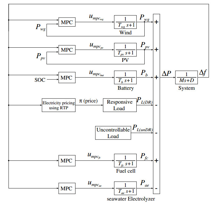
This work presents a load frequency control scheme in Renewable Energy Sources(RESs) power system by applying Model Predictive Control(MPC). The MPC is designed depending on the first model parameter and then investigate its performance on the second model to confirm its robustness and effectiveness over a wide range of operating conditions. The first model is 100% RESs system with Photovoltaic generation(PV), wind generation(WG), fuel cell, seawater electrolyzer, and storage battery. From the simulation results of the first case, it shows the control scheme is efficiency. And base on the good results of the first case study, to propose a second case using a 10-bus power system of Okinawa island, Japan, to verify the efficiency of proposed MPC control scheme again. In addition, in the second case, there also applied storage devices, demand-response technique and RESs output control to compensate the system frequency balance. Last, there have a detailed results analysis to compare the two cases simulation results, and then to Prospects for future research. All the simulations of this work are performed in Matlab®/Simulink®.
Citation: Lei Liu, Takeyoshi Kato, Paras Mandal, Alexey Mikhaylov, Ashraf M. Hemeida, Hiroshi Takahashi, Tomonobu Senjyu. Two cases studies of Model Predictive Control approach for hybrid Renewable Energy Systems[J]. AIMS Energy, 2021, 9(6): 1241-1259. doi: 10.3934/energy.2021057
This work presents a load frequency control scheme in Renewable Energy Sources(RESs) power system by applying Model Predictive Control(MPC). The MPC is designed depending on the first model parameter and then investigate its performance on the second model to confirm its robustness and effectiveness over a wide range of operating conditions. The first model is 100% RESs system with Photovoltaic generation(PV), wind generation(WG), fuel cell, seawater electrolyzer, and storage battery. From the simulation results of the first case, it shows the control scheme is efficiency. And base on the good results of the first case study, to propose a second case using a 10-bus power system of Okinawa island, Japan, to verify the efficiency of proposed MPC control scheme again. In addition, in the second case, there also applied storage devices, demand-response technique and RESs output control to compensate the system frequency balance. Last, there have a detailed results analysis to compare the two cases simulation results, and then to Prospects for future research. All the simulations of this work are performed in Matlab®/Simulink®.

| [1] | Stott PA, Mueller MA (2006) Modelling fully variable speed hybrid wind diesel systems. Proceedings of the 41st International Universities Power Engineering Conference, 9486735, Newcastle upon Tyne, UK. |
| [2] | Alternative Energy Solutions for the 21st Century, Renewable Energy. [Online]. Available from: http://www.altenergy.org/renewables/renewables.htmll. |
| [3] | Vazquez S, Rodriguez J, Rivera M, et al. (2016) Model eredictive control for power converters and drives: Advances and trends. IEEE Trans Ind Electron 64: 935-947. |
| [4] | Serale G, Fiorentini M, Capozzoli A, et al. (2018) Model Predictive Control (MPC) for enhancing building and HVAC system energy efficiency: Problem formulation, applications and opportunities. Energies 11: 631. |
| [5] | Lu K, Zhou W, Zeng G, et al. (2019) Constrained population extremal optimization-based robust load frequency control of multi-area interconnected power system. Int J Electr Power Energy Syst 105: 249-271. |
| [6] | Al-Ghussain L, Ahmed H, Haneef F (2018) Optimization of hybrid PV-wind system: Case study Al-Tafilah cement factory, Jordan. Sustainable Energy Technol Assess 30: 24-36. |
| [7] | Mazzeo D, Matera N, De Luca P, et al. (2021) A literature review and statistical analysis of photovoltaic-wind hybrid renewable system research by considering the most relevant 550 articles: An upgradable matrix literature database. J Cleaner Prod 295: 126070. |
| [8] | Anoune K, Laknizia A, Bouyaa M, et al. (2018) Sizing a PV-Wind based hybrid system using deterministic approach. Energy Convers Manage 169: 137-148. |
| [9] | Mazzeo D, Matera N, Oliveti G (2018) Interaction between a wind-PV-battery-heat pump trigeneration system and office building electric energy demand including vehicle charging. 2018 IEEE International Conference on Environment and Electrical Engineering and 2018 IEEE Industrial and Commercial Power Systems Europe (EEEIC/ICPS Europe) 18182476, Palermo, Italy. |
| [10] | Mazzeo D, Herdem MS, Matera N, et al. (2021) Artificial intelligence application for the performance prediction of a clean energy community. Energy 232: 120999. |
| [11] | Acuna LG, Padilla RV, Mercado AS (2016) Measuring reliability of hybrid photovoltaic-wind energy systems: A new indicator. Renewable Energy 8426: 152-178. |
| [12] | Zhao C, Mallada E, Low SH, et al. (2018) Distributed plug-and-play optimal generator and load control for power system frequency regulation. Int J Electr Power Energy Syst 101: 1-12. |
| [13] | Babahajiani P, Shafiee Q, Bevrani H (2016) Intelligent demand response contribution in frequency control of Multi-Area power systems. IEEE Trans Smart Grid 9: 1282-1291. |
| [14] | Bahrami S, Sheikhi A (2015) From demand response in smart grid toward integrated demand response in smart energy hub. IEEE Trans Smart Grid 7: 650-658. |
| [15] | Vardakas JS, Zorba N, Verikoukis CV (2014) A Survey on demand response programs in smart grids: Pricing methods and optimization algorithms. IEEE Commun Surv Tutorials 17: 152-178. |


Figures(27) / Tables(5)

Lei Liu, Takeyoshi Kato, Paras Mandal, Alexey Mikhaylov, Ashraf M. Hemeida, Hiroshi Takahashi, Tomonobu Senjyu. Two cases studies of Model Predictive Control approach for hybrid Renewable Energy Systems[J]. AIMS Energy, 2021, 9(6): 1241-1259. doi: 10.3934/energy.2021057


 DownLoad: