Loading [MathJax]/jax/output/SVG/jax.js
Research article Special Issues

A life cycle inventory analysis of wood pellets for greenhouse heating: a case study at Macdonald campus of McGill University1

  • Received: 10 July 2016 Accepted: 22 September 2016 Published: 29 September 2016
  • Wood pellets are one of the most promising alternatives to fossil fuel in Canada. Using wood pellets for heating allows saving on heating source expenses as compared to fossil fuels. Moreover, direct carbon emissions from wood pellets are regarded as carbon neutral since regrowth of vegetation captures and stores carbon that already exists in the atmosphere. Using wood pellets as a heating fuel for greenhouse vegetable production is expected to result in less greenhouse gas emissions than fossil fuels. Increasing the domestic consumption of wood pellets for greenhouse heating in Canada would reduce the environmental impact of energy consumption. This study investigates the potential of using wood pellets as an alternative fuel for commercial greenhouses in Quebec. This study applied a life-cycle analysis to demonstrate the energy flows and environmental consequences of using wood pellets for greenhouse vegetable production. The results found that greenhouse gas emissions from wood pellets are lower than natural gas in greenhouse operations.

    Citation: Tingting Wu, Kakali Mukhopadhyay, Paul J. Thomassin. A life cycle inventory analysis of wood pellets for greenhouse heating: a case study at Macdonald campus of McGill University1[J]. AIMS Energy, 2016, 4(5): 697-722. doi: 10.3934/energy.2016.5.697

    Related Papers:

    [1] Xian Hua, Jing Li, Ting Wang, Junhong Wang, Shaojun Pi, Hangcheng Li, Xugang Xi . Evaluation of movement functional rehabilitation after stroke: A study via graph theory and corticomuscular coupling as potential biomarker. Mathematical Biosciences and Engineering, 2023, 20(6): 10530-10551. doi: 10.3934/mbe.2023465
    [2] Hongming Liu, Yunyuan Gao, Wei Huang, Rihui Li, Michael Houston, Julia S. Benoit, Jinsook Roh, Yingchun Zhang . Inter-muscular coherence and functional coordination in the human upper extremity after stroke. Mathematical Biosciences and Engineering, 2022, 19(5): 4506-4525. doi: 10.3934/mbe.2022208
    [3] Teng Li, Xiang Chen, Shuai Cao, Xu Zhang, Xun Chen . Human hands-and-knees crawling movement analysis based on time-varying synergy and synchronous synergy theories. Mathematical Biosciences and Engineering, 2019, 16(4): 2492-2513. doi: 10.3934/mbe.2019125
    [4] Konki Sravan Kumar, Daehyun Lee, Ankhzaya Jamsrandoj, Necla Nisa Soylu, Dawoon Jung, Jinwook Kim, Kyung Ryoul Mun . sEMG-based Sarcopenia risk classification using empirical mode decomposition and machine learning algorithms. Mathematical Biosciences and Engineering, 2024, 21(2): 2901-2921. doi: 10.3934/mbe.2024129
    [5] Baohua Hu, Yong Wang, Jingsong Mu . A new fractional fuzzy dispersion entropy and its application in muscle fatigue detection. Mathematical Biosciences and Engineering, 2024, 21(1): 144-169. doi: 10.3934/mbe.2024007
    [6] Xiebing Chen, Yuliang Ma, Xiaoyun Liu, Wanzeng Kong, Xugang Xi . Analysis of corticomuscular connectivity during walking using vine copula. Mathematical Biosciences and Engineering, 2021, 18(4): 4341-4357. doi: 10.3934/mbe.2021218
    [7] Qun Xu, Suqi Xue, Farong Gao, Qiuxuan Wu, Qizhong Zhang . Evaluation method of motor unit number index based on optimal muscle strength combination. Mathematical Biosciences and Engineering, 2023, 20(2): 3854-3872. doi: 10.3934/mbe.2023181
    [8] Shaojun Zhu, Jinhui Zhao, Yating Wu, Qingshan She . Intermuscular coupling network analysis of upper limbs based on R-vine copula transfer entropy. Mathematical Biosciences and Engineering, 2022, 19(9): 9437-9456. doi: 10.3934/mbe.2022439
    [9] Liangyu Yang, Tianyu Shi, Jidong Lv, Yan Liu, Yakang Dai, Ling Zou . A multi-feature fusion decoding study for unilateral upper-limb fine motor imagery. Mathematical Biosciences and Engineering, 2023, 20(2): 2482-2500. doi: 10.3934/mbe.2023116
    [10] Chengliang Wu, Weiya Hao, Wei He, Xiaofei Xiao, Xuhong Li, Wei Sun . Biomechanical and neuromuscular strategies on backward somersault landing in artistic gymnastics: A case study. Mathematical Biosciences and Engineering, 2019, 16(5): 5862-5876. doi: 10.3934/mbe.2019293
  • Wood pellets are one of the most promising alternatives to fossil fuel in Canada. Using wood pellets for heating allows saving on heating source expenses as compared to fossil fuels. Moreover, direct carbon emissions from wood pellets are regarded as carbon neutral since regrowth of vegetation captures and stores carbon that already exists in the atmosphere. Using wood pellets as a heating fuel for greenhouse vegetable production is expected to result in less greenhouse gas emissions than fossil fuels. Increasing the domestic consumption of wood pellets for greenhouse heating in Canada would reduce the environmental impact of energy consumption. This study investigates the potential of using wood pellets as an alternative fuel for commercial greenhouses in Quebec. This study applied a life-cycle analysis to demonstrate the energy flows and environmental consequences of using wood pellets for greenhouse vegetable production. The results found that greenhouse gas emissions from wood pellets are lower than natural gas in greenhouse operations.


    Nonlinear partial differential equations (PDEs) are often used to describe some significant problems in natural science and engineering technology. The analysis of nonlinear waves has garnered increasing attention in the fields of shallow water, plasma, nonlinear optics, Bose−Einstein condensates, and fluids. The nonlinear PDEs in these fields can be solved using lump solutions. The lump solution and interaction hybrid solutions were first discovered by Zakharov in [1] and Craik in [2], respectively. These special solutions are of great significance for the study of nonlinear integrable equations [3,4,5]. To obtain these analytical solutions, the scholars have proposed a variety of methods, including Ansatz technique [6], Hirota's bilinear method (HBM) [7], and the inverse scattering transform (IST) [8]. The HBM proposed by Hirota, has been widely used as an effective approach to study the nonlinear dynamics wave equation, resulting in numerous richer solutions, such as solitons solutions, novel breather waves, lump solutions, two-wave solutions, and rogue wave solutions ([9,10,11,12,13,14]). These solutions are visualized in three-dimensional graphics via numerical simulations, making it easier to understand the propagation of nonlinear waves.

    The study of the stability of integrable equations, such as the KPI equation, the Ishimori equation, the nonlinear Schrödinger (NLS) equation and the KdV equation have further enriched the theory of nonlinear wave equations. Spectral methods can effectively solve the problem of linear stability. In [15], Degasperis et al. proposed the construction of the eigenmodes of the linearized equation using the associated Lax pair and provided the computation of both analytical and numerical solutions with the example of two coupled NLS equations. In [16], Ablowitz provided a comprehensive review of research methods for integrability and nonlinear waves, including Bäcklund transformations, Darboux transformations, direct integral equations or Riemann−Hilbert or Dbar methods, and HBM. By combining the KdV and NLS equations, the author further elaborated on the ideas and background of the IST method.

    The computation of nonlinear PDEs has become a very active research topic. With advancements in traditional methods like finite element ([17,18]), finite difference ([19,20,21,22,23,24]), finite volume ([25,26,27]), and spectral methods ([28,29,30]), numerous outstanding research results have been achieved in the numerical approximations of nonlinear PDEs. In [31], the authors developed a time-two-grid difference scheme for nonlinear Burgers equations. In [32], a method combining the barycentre Lagrange interpolation collocation technique with a second-order operator splitting approach was proposed for the purpose of solving the NLS equation. Based on novel shifted Delannoy functions, Ansari et al. [33] employed a matrix collocation technique to numerically approximate the singularly perturbed parabolic convection−diffusion−reaction problems.

    In recent years, for the treatment of nonlinear terms, there have been a lot of unconditionally energy dissipative numerical schemes for Allen−Cahn and Cahn−Hilliard gradient flows models, such as:

    (ⅰ) CSS (convex splitting) scheme [34,35,36];

    (ⅱ) IMEX (stabilized semi-implicit) scheme [37,38];

    (ⅲ) ETD (exponential time differencing) scheme [39,40];

    (ⅳ) IEQ (invariant energy quadratization) scheme [41];

    (ⅴ) SAV (scalar auxiliary variable) scheme [42,43];

    (ⅵ) E-SAV (exponential scalar auxiliary variable) scheme [44].

    The idea of (ⅰ) is to decompose the energy function into convex and concave parts, handling the convex part implicitly and the concave part explicitly. The advantage is that it can achieve second-order unconditional stability. However, the drawback is that it still requires solving nonlinear equations. The method of (ⅱ) yields extra error, which makes it difficult to construct a higher-order scheme. The (ⅳ) and (ⅴ) approaches make it easier to handle nonlinear terms by defining auxiliary variables that transform the nonlinear potential function into a simple quadratic form. Nevertheless, an inner product must be calculated before obtaining the next time value. Compared with (ⅳ) and (ⅴ), the variable defined in (ⅵ) does not require any assumptions. And the E-SAV method can easily construct an explicit scheme that can preserve energy stability. But this physical property can not be satisfied with the explicit SAV scheme.

    In addition, Huang et al. [45] studied a new SAV method to approximate the gradient flows, which is an improvement of the SAV method. By defining an auxiliary variable in the new SAV method as a shifted total energy function, instead of focusing on the nonlinear parts of the classic SAV method, we replace the dynamic equation for that variable with the energy balance equation of the gradient flow. This facilitates the construction of high-order and energy-stable discrete schemes. In [46], Liu et al. further developed an exponential semi-implicit scalar auxiliary variable (ESI-SAV) method for the phase field equation. The ESI-SAV method can preserve the advantages of both the new SAV and E-SAV methods and be applied more effectively to other dissipative systems.

    On the basis of the above methods, researchers began to apply the above nonlinear processing techniques to approximate semi-linear wave equations. Jiang et al. [47] proposed an IEQ approach and established an energy-preserving linear implicit scheme for the sine-Gordon equation. In [48], based on the SAV method with a combination of the Gauss technique and the extrapolation method, Li et al. provided a high-order energy-conserving and linearly implicit scheme. Wang et al. [49] developed a second-order SAV Fourier spectral method to solve a nonlinear fractional generalized wave equation.

    The primary objective of this paper is to develop second-order and Hamiltonian conserved semi-discrete schemes for semi-linear wave equations. Following the superiorities of the E-SAV and ESI-SAV methods, two different numerical schemes are given by utilizing the Crank−Nicolson scheme for temporal approximation. Furthermore, the convergence order and the evolution curve of the Hamiltonian function are validated through numerical experiments.

    The paper is organized as follows: In Section 2, by introducing scalar auxiliary variables, we obtain two equivalent forms for the semi-linear wave equation in the continuous case. In Sections 3 and 4, by using the Crank−Nicolson scheme, we propose two semi-discrete schemes corresponding to the equivalent forms and provide proof of the convergence order. Two numerical examples are implemented to test the effectiveness of the theoretical analysis in Section 5.

    We consider the following semi-linear wave equation:

    {yttΔyf(y)=0,xΩ,t(0,T),y(x,t)=0,xΩ,t(0,T),y(x,0)=y0(x),yt(x,0)=g(x),xΩ, (2.1)

    where ΩRd(d=2,3) is a bounded convex domain, T>0 is a fixed number, f(y)=F(y) is a nonlinear term, and F(y) satisfies F(y)C3(R). The Hamiltonian function is defined as

    H(y)=12||yt||2+12||y||2+ΩF(y)dx. (2.2)

    Proposition 2.1. The system (2.1) holds the following Hamiltonian conservation law:

    dH(y)dt=0. (2.3)

    Proof. Multiplying the first equation of the system (2.1) by yt yields

    yttytΔyytf(y)yt=0. (2.4)

    By using the continuous Leibniz rule, we obtain

    yttyt=12((yt)2)t,f(y)yt=(F(y))t, (2.5)

    and

    Δyyt=(yx1x1+yx2x2)yt=(yx1yt)x1+(yx2yt)x2yx1(yt)x1yx2(yt)x2=(yx1yt)x1+(yx2yt)x212(y2x1+y2x2)t. (2.6)

    Inserting (2.5) and (2.6) into (2.4), we obtain

    [12((yt)2)t+12(y2x1+y2x2)t+(F(y))t][(yx1yt)x1+(yx2yt)x2]=0. (2.7)

    Integrating (2.7) over the spatial domain Ω and combining the boundary conditions leads to

    Ω[12((yt)2)t+12(y2x1+y2x2)t+(F(y))t]dx=0, (2.8)

    From (2.8) and (2.2), we can deduce that

    dH(y)dt=Ω[12((yt)2)t+12(y2x1+y2x2)t+(F(y))t]dx=0. (2.9)

    The proof is complete.

    We introduce two scalar auxiliary variables as

    ω=yt,r(t)=ΩF(y)dx=H2(y).

    Then the system (2.1) can be equivalently rewritten as

    ω=yt,xΩ,t(0,T), (2.10)
    ωtΔyqy,rf(y)=0,xΩ,t(0,T), (2.11)
    rt=qy,r(f(y),ω),xΩ,t(0,T), (2.12)
    y(x,t)=0,ω(x,t)=0,xΩ,t(0,T), (2.13)
    y(x,0)=y0(x),ω(x,0)=g(x),r(0)=H2(y0(x)),xΩ, (2.14)

    where

    qy,r=exp{r}exp{H2(y)}.

    For the system (2.10)–(2.14), we have the following lemma:

    Lemma 2.1. (Hamiltonian conservation) The above system (2.10)–(2.14) satisfies

    d˜H(y)dt=0, (2.15)

    where the modified Hamiltonian function

    ˜H(t)=12||ω||2+12||y||2+r. (2.16)

    Proof. Taking the inner product of (2.11) by ω, then combining (2.10) and (2.12), we obtain

    (ωt,ω)+(y,yt)+rt=0.

    Obviously, we can deduce

    ddt(12||ω||2+12||y||2+r)=0.

    The proof is complete.

    Next, introducing a new variable

    R(t)=H(y),

    which satisfies the dissipation law

    dRdt=dH(y)dt=0, (2.17)

    and defining ξ=exp(R)exp(H(y)), we can know that ξ1 in the continuous case. Replacing the factor qy,r in (2.11) by Q(ξ), where Q(ξ) is a polynomial function of ξ, the system (2.1) can be transformed into the following equivalent form:

    ω=yt,xΩ,t(0,T), (2.18)
    ωtΔyQ(ξ)f(y)=0,xΩ,t(0,T), (2.19)
    ξ=exp(R)exp(H(y))xΩ,t(0,T), (2.20)
    Q(ξ)=ξ(2ξ)xΩ,t(0,T), (2.21)
    dRdt=0,xΩ,t(0,T), (2.22)
    y(x,t)=0,ω(x,t)=0,xΩ,t(0,T), (2.23)
    y(x,0)=y0(x),ω(x,0)=g(x),R(0)=H(y0),xΩ. (2.24)

    Furthermore, (2.17) and (2.22) imply that the system (2.18)–(2.24) is Hamiltonian conserved.

    Let 0=t0<t1<...<tN=T be a uniform partition of the time interval [0,T] with the time steps Δt=T/N and tn=nΔt. Then, utilizing the Crank−Nicolson scheme to discretize the system (2.10)–(2.14), a second-order Carnk−Nicolson E-SAV (CN-E-SAV) scheme can be formulated as follows:

    ωn+12=1Δt(yn+1yn), (3.1)
    1Δt(ωn+1ωn)Δyn+12ˆqn+12f(ˆyn+12)=0, (3.2)
    1Δt(rn+1rn)=(ˆqn+12f(ˆyn+12),ωn+12), (3.3)

    where

    ωn+12=12(ωn+1+ωn),yn+12=12(yn+1+yn),

    and ˆqn+12>0 with (ˆyn+12,ˆrn+12) being generated by the first-order scheme with the time step size Δt2, i.e.,

    ˆωn+12=1Δt/2(ˆyn+12yn), (3.4)
    1Δt/2(ˆωn+12ωn)Δˆyn+12qnf(yn)=0, (3.5)
    1Δt/2(ˆrn+12rn)=qn(f(yn),ˆωn+12). (3.6)

    In order to better understand this scheme, by plugging (3.1) into (3.2) and (3.4) into (3.5), respectively, we can get

    2Δt2yn+112Δyn+1=2Δt2yn+2Δtωn+12Δyn+ˆqn+12f(ˆyn+12), (3.7)
    4Δt2ˆyn+12Δˆyn+12=4Δt2yn+2Δtωn+qnf(yn). (3.8)

    So we can implement the CN-E-SAV scheme as follows:

    (i). Computeqnfromqn=exp{rn}exp{H2(yn)};(ii). Computeˆyn+12from(3.8);(iii). Computeˆωn+12from(3.4);(iv). Computeˆrn+12from(3.6);(v). Computeˆqn+12fromˆqn+12=exp{ˆrn+12}exp{H2(ˆyn+12)};(vi). Computeyn+1from(3.7);(vii). Computeωn+1from(3.1);(viii). Computern+1from(3.3).

    We show the conservation of the CN-E-SAV scheme by the following theorem:

    Theorem 3.1. The CN-E-SAV scheme (3.1)–(3.3) is Hamiltonian conserved:

    Hn+1=HnwithHn=12||ωn||2+12||yn||2+rn. (3.9)

    Proof. Taking the inner product with (3.1) and (3.2) by yn+12, ωn+12, we have

    (ωn+12,yn+12)=12Δt||yn+1||212Δt||yn||2, (3.10)

    and

    12||ωn+1||212||ωn||2+Δt(yn+12,ωn+12)ˆqn+12(f(ˆyn+12),ωn+12)Δt=0. (3.11)

    Substituting (3.10) into (3.11) and combining (3.3), we obtain

    (12||ωn+1||2+12||yn+1||2+rn+1)(12||ωn||2+12||yn||2+rn)=0.

    The proof is complete.

    We will follow the next two steps to complete the error estimation of the CN-E-SAV scheme:

    step (ⅰ): complete the error between (2.10)–(2.14) and (3.4)–(3.6);

    step (ⅱ): with the help of the results of step (ⅰ), the error of (2.10)–(2.14) and (3.1)–(3.3) is further estimated.

    For simplicity, we define

    ˆen+12ω=ω(tn+12)ˆωn+12,enω=ω(tn)ωn,ˆen+12y=y(tn+12)ˆyn+12,eny=y(tn)yn,ˆen+12r=r(tn+12)ˆrn+12,enr=r(tn)rn.

    It follows from (2.10)–(2.14) that the exact solution (ω,y,r) satisfies

    ω(tn+12)=1Δt/2(y(tn+12)y(tn))1Δt/2ˆTny1, (3.12)
    ω(tn+12)ω(tn)Δt/2Δy(tn+12)q(tn)f(y(tn))=1Δt/2ˆTnωΔ(y(tn+12)y(tn)), (3.13)
    r(tn+12)r(tn)=(q(tn)f(y(tn)),y(tn+12)y(tn)ˆTny2)+ˆTnr, (3.14)

    where the truncation functions are defined as

    ˆTnω=tn+12tn(tn+12t)ωttdt,ˆTny1=tn+12tn(tnt)yttdt,ˆTny2=tn+12tn(tn+12t)yttdt,ˆTnr=tn+12tn(tn+12t)rttdt,

    and satisfy

    ||ˆTnω||2C(Δt)3tn+12tn||ωtt||2dt,||ˆTny1||2C(Δt)3tn+12tn||ytt||2dt, (3.15)
    ||ˆTny2||2C(Δt)3tn+12tn||ytt||2dt,|ˆTnr|2C(Δt)3tn+12tn|rtt|2dt. (3.16)

    For the purposes of theorem proving, we present the following assumptions and lemmas:

    Assumption 3.1. There exist constants Q, Q, ˜Q, and ˜Q independent of Δt such that QqnQ, ˜Qˆqn+12˜Q for all n.

    Lemma 3.1. Denote

    A=q(tn)f(y(tn))qnf(yn),B=ˆqn+12f(ˆyn+12)q(tn+12)f(y(tn+12)),

    then the following holds:

    ||A||C(||eny||+|enr|),||B||C(||ˆen+12y||+|ˆen+12r|),

    where the constant C>0 depends on Q,Q,˜Q, ˜Q,|Ω|,y0, and ||f||C1(R).

    Proof. Similar to the proof of Lemma 4 of [51], the results can be proved by applying Poincaré's inequality to ||eny||,||ˆen+12y|| once more.

    Lemma 3.2. Assume Δt is sufficiently small and satisfies

    ytL(0,T;L2)L2(0,T;H2),yttL2(0,T;L2)L2(0,T;H1),ytttL2(0,T;L2).

    Then, we have

    ||ˆen+12ω||2+||ˆen+12y||2+|ˆen+12r|2ˇC(Δt)3tn+12tn(||ωtt||2+||ytt||2+|rtt|2+||ytt||2+||yt||2H2(Ω))ds+ˇC(||enω||2+||eny||2+|enr|2). (3.17)

    Proof. Subtracting (3.4)–(3.6) from (3.12)–(3.14), we have the error equations as

    ˆen+12ω=1Δt/2(ˆen+12yeny)1Δt/2ˆTny1, (3.18)
    ˆen+12ωenωΔt/2Δˆen+12y=q(tn)f(y(tn))qnf(yn)Δ(y(tn+12)y(tn))+1Δt/2ˆTnω, (3.19)
    ˆen+12renr=(qnf(yn),ˆen+12yeny)+(qnf(yn)q(tn)f(y(tn)),y(tn+12)y(tn))+(q(tn)f(y(tn)),ˆTny2)+ˆTnr. (3.20)

    Taking the inner product of (3.19) with ˆen+12ω and combining (3.18), we have

    ||ˆen+12ω||2||enω||2+||ˆen+12ωenω||2+||ˆen+12y||2||eny||2+||(ˆen+12yeny)||2=Δt(A,ˆen+12ω)Δt(Δ(y(tn+12)y(tn)),ˆen+12ω)+2(ˆTnω,ˆen+12ω)2(ˆTny1,Δˆen+12y):=Λ1+Λ2+Λ3+Λ4. (3.21)

    For the first term on the right-hand side of (3.21), according to Lemma 3.1, we obtain

    Λ1C(Δt)2||A||2+14||ˆen+12ω||2˜C1(Δt)2(||eny||2+|enr|2)+14||ˆen+12ω||2. (3.22)

    Then for Λ2,Λ3,Λ4, using Young's inequality and (3.15), one has

    Λ2C(Δt)3tn+12tn||yt||2H2(Ω)ds+14||ˆen+12ω||2, (3.23)
    Λ3C(Δt)3tn+12tn||ωtt||2dt+14||ˆen+12ω||2, (3.24)
    Λ4C(Δt)3tn+12tn||ytt||2dt+14||ˆen+12y||2. (3.25)

    Combining (3.22)–(3.25) with (3.21), we can have

    ||ˆen+12ω||2+4||ˆen+12ωenω||2+||ˆen+12y||2+4||(ˆen+12yeny)||24˜C1(Δt)2(||eny||2+|enr|2)+4(||enω||2+||eny||2)+C(Δt)3tn+12tn(||ωtt||2+||ytt||2+||yt||2H2(Ω))ds. (3.26)

    Multiplying (3.20) by ˆen+12r, we can obtain

    |ˆen+12r|2|enr|2+|ˆen+12renr|2=2(qnf(yn),ˆen+12yeny)ˆen+12r2(A,y(tn+12)y(tn))ˆen+12r+2(q(tn)f(y(tn)),ˆTny2)ˆen+12r+2ˆTnrˆen+12r:=Ψ1+Ψ2+Ψ3+Ψ4. (3.27)

    According to qnQ,FC3(R), and Poincaré's inequality, we can derive the following estimate for Ψ1:

    Ψ1||qnf(yn)||||ˆen+12yeny|||ˆen+12r|C||(ˆen+12yeny)||2+14|ˆen+12r|2. (3.28)

    The estimate for Ψ2 is similar to (3.22), so we obtain

    Ψ2Δt||A||||y(tn+12)y(tn)Δt|||ˆen+12r|˜C2(Δt)2(||eny||2+|enr|2)+14|ˆen+12r|2. (3.29)

    For the last two terms of (3.27), by utilizing (3.16), we have that

    Ψ3+Ψ4C(Δt)3tn+12tn(|rtt|2+||ytt||2)ds+14|ˆen+12r|2. (3.30)

    Therefore, injecting (3.28)–(3.30) into (3.27) leads to

    |ˆen+12r|2+4|ˆen+12renr|24˜C2(Δt)2(||eny||2+|enr|2)+C(Δt)3tn+12tn(|rtt|2+||ytt||2)dt+4C||(ˆen+12yeny)||2+4|enr|2. (3.31)

    Multiplying (3.26) by C and adding it to (3.31) implies

    C||ˆen+12ω||2+C||ˆen+12y||2+|ˆen+12r|24(˜C1C+˜C2)(Δt)2(||eny||2+|enr|2)+4C(||enω||2+||eny||2)+4|enr|2+C(Δt)3tn+12tn(||ωtt||2+||ytt||2+|rtt|2+||ytt||2+||yt||2H2(Ω))ds.

    The proof is completed when C1 and (Δt)2C˜C1C+˜C2.

    Next, we will derive the convergence order of the CN-E-SAV scheme (3.1)–(3.3). Clearly, the exact solution (ω,y,r) satisfies

    ω(tn+1)+ω(tn)2=1Δt(y(tn+1)y(tn))+Rnω1ΔtTny, (3.32)
    1Δt(ω(tn+1)ω(tn))Δy(tn+1)+y(tn)2q(tn+12)f(y(tn+12))=1ΔtTnωΔRny, (3.33)
    1Δt(r(tn+1)r(tn))=(q(tn+12)f(y(tn+12)),ω(tn+1)+ω(tn)2Rω)+1ΔtTnr, (3.34)

    where the truncation functions are defined by

    Tω=ω(tn+1)ω(tn)Δtωt(tn+12),Ty=y(tn+1)y(tn)Δtyt(tn+12),Tr=r(tn+1)r(tn)Δtrt(tn+12),Rω=ω(tn+1)+ω(tn)2ω(tn+12),Ry=y(tn+1)+y(tn)2y(tn+12),Rr=r(tn+1)+r(tn)2r(tn+12).

    The truncation functions satisfy the following lemma:

    Lemma 3.3. ([50]) The following estimates hold

    ||Tω||2C(Δt)5tn+1tn||ωttt||2ds,||Ty||2C(Δt)5tn+1tn||yttt||2ds,|Tr|2C(Δt)5tn+1tn|rttt|2ds,||Rω||2C(Δt)3tn+1tn||ωtt||2ds,||Ry||2C(Δt)3tn+1tn||ytt||2ds,|Rr|2C(Δt)3tn+1tn|rtt|2ds.

    Theorem 3.2. Let (ω(tn),y(tn),r(tn)) and (ωn,yn,rn) be the solutions of (2.10)–(2.14) and CN-E-SAV scheme (3.1)–(3.3), respectively. Suppose that the assumptions in Lemma 3.2 hold and assume further

    yttL2(0,T;L2)L2(0,T;H2),ytttL2(0,T;L2)L2(0,T;H1),yttttL2(0,T;L2).

    Then, we have

    ||enω||2+||eny||2+|enr|2C(Δt)4.

    Proof. Subtracting (3.1)–(3.3) from (3.32)–(3.34), we derive the following error equations:

    en+12ω=1Δt(en+1yeny)+Rnω1ΔtTny, (3.35)
    1Δt(en+1ωenω)Δen+12y=q(tn+12)f(y(tn+12))ˆqn+12f(ˆyn+12)+1ΔtTnωΔRny, (3.36)
    1Δt(en+1renr)=(ˆqn+12f(ˆyn+12)q(tn+12)f(y(tn+12)),ω(tn+1)+ω(tn)2)(ˆqn+12f(ˆyn+12),en+12ω)+(q(tn+12)f(y(tn+12)),Rnω)+1ΔtTnr. (3.37)

    Taking the inner product of (3.36) with en+12ω and combining (3.35), we have

    12||en+1ω||212||enω||2+12||en+1y||212||eny||2=Δt(B,en+12ω)+(Tnω,en+12ω)Δt(ΔRny,en+12ω)Δt(en+12y,Rnω)Δt(en+12y,Tny):=Υ1+Υ2+Υ3+Υ4+Υ5. (3.38)

    According to Lemma 3.1, we obtain

    Υ1CΔt(|ˆen+12r|2+||ˆen+12y||2+||en+12ω||2). (3.39)

    For the last four terms of (3.38), it follows from Lemma 3.3 that

    Υ2C(Δt)4tn+1tn||ωttt||2dt+CΔt||en+12ω||2, (3.40)
    Υ3C(Δt)4tn+1tn||Δytt||2dt+CΔt||en+12ω||2, (3.41)
    Υ4C(Δt)4tn+1tn||ωtt||2dt+CΔt||en+12y||2, (3.42)
    Υ5C(Δt)4tn+1tn||yttt||2dt+CΔt||en+12y||2. (3.43)

    Substituting (3.39)–(3.43) into (3.38), we can obtain

    12||en+1ω||212||enω||2+12||en+1y||212||eny||2CΔt(|ˆen+12r|2+||ˆen+12y||2)+CΔt(||en+12ω||2+||en+12y||2)+C(Δt)4tn+1tn(||ωttt||2+||yttt||2+||Δytt||2+||ωtt||2)dt. (3.44)

    Multiplying (3.3) by en+12r, we obtain

    12(|en+1r|2|enr|2)=Δten+12r(B,ω(tn+1)+ω(tn)2)Δten+12r(ˆqn+12f(ˆyn+12),en+12ω)+Δt(q(tn+12)f(y(tn+12)),Rnω)en+12r+Tnren+12r:=Φ1+Φ2+Φ3+Φ4. (3.45)

    Next, we estimate the right-hand side of (3.45). Applying Lemma 3.1, Lemma 3.3, and Young's inequality, we deduce that

    Φ1CΔt|en+12r|||B||||ω(tn+1)+ω(tn)2||CΔt(|ˆen+12r|2+||ˆen+12y||2+|en+12r|2), (3.46)
    Φ2CΔt(|en+12r|2+||en+12ω||2), (3.47)
    Φ3+Φ4C(Δt)4tn+1tn(||ωtt||2+|rttt|2)dt+CΔt|en+12r|2. (3.48)

    Combining the above estimates of (3.46)–(3.48) together, one has

    12|en+1r|212|enr|2CΔt(|ˆen+12r|2+||ˆen+12y||2)+CΔt(||en+12ω||2+|en+12r|2)+C(Δt)4tn+1tn(||ωtt||2+|rttt|2)dt. (3.49)

    By adding (3.44) and (3.49) and summing the index k from 0 to n1, we obtain

    ||enω||2+||eny||2+||enr||2CΔtn1k=0(||ekω||2+||eky||2+|ekr|2)+CΔtn1k=0(|ˆek+12r|2+||ˆek+12y||2)+C(Δt)4tn0(||ωttt||2+|rttt|2+||yttt||2+||ωtt||2+||ytt||2+|rtt|2+||Δytt||2+||ωtt||2)dt.

    Applying Lemma 3.2 and the discrete Gronwall's inequality, we can complete the proof.

    For the system (2.18)–(2.24), we obtain the semi-discrete new Crank−Nicolson E-SAV (New-CN-E-SAV) scheme by adopting the Crank−Nicolson scheme as

    ωn+1+ωn2=1Δt(yn+1yn), (4.1)
    1Δt(ωn+1ωn)Δyn+1+yn2Q(ξn+1)f(ˆyn+12)=0, (4.2)
    ξn+1=exp(Rn+1)exp(H(ˆyn+12)), (4.3)
    Q(ξn+1)=ξn+1(2ξn+1), (4.4)
    1Δt(Rn+1Rn)=0, (4.5)

    where ˆyn+12 is obtained by solving the following equation:

    ˆwn+12=1Δt/2(ˆyn+12yn), (4.6)
    1Δt/2(ˆωn+12ωn)Δˆyn+12f(yn)=0. (4.7)

    From (4.5), we can find that the New-CN-E-SAV scheme (4.1)–(4.5) also enjoys the same conservation as the CN-E-SAV scheme (3.1)–(3.3).

    Theorem 4.1. The New-CN-E-SAV scheme (4.1)–(4.5) is Hamiltonian conserved in the sense that

    Rn+1=Rn==R0.

    Further, according to Theorem 4.1, the Eq (4.3) can be simplified as

    ξn+1=exp(R0)exp(H(ˆyn+12)). (4.8)

    In order to better illustrate the calculation process of the New-CN-E-SAV scheme (4.1)–(4.5), plugging (4.1) and (4.6) into (4.2) and (4.7), respectively, we obtain

    (2Δt212Δ)yn+1=2Δt2yn+2Δtωn+12Δyn+Q(ξn+1)f(ˆyn+12), (4.9)
    (4Δt2Δ)ˆyn+12=4Δt2yn+2Δtωn+f(yn). (4.10)

    So the New-CN-E-SAV scheme can be implemented as follows:

    (i). solveˆyn+12from(4.10);(ii). solveˆωn+12from(4.6);(iii). computeξn+1from(4.8);(iv). computeQ(ξn+1)from(4.4);(v). solveyn+12from(4.9);(vi). solveωn+12from(4.1).

    For the convergence order of the New-CN-E-SAV scheme, from (4.6) and (4.7), we can obtain

    ˆyn+12=y(tn+12)+O(Δt2), (4.11)
    ˆωn+12=ω(tn+12)+O(Δt2). (4.12)

    Referring to [46] and combining (4.11) and (4.12), we obtain

    ξn+1=exp(R0)exp(H(ˆyn+12))=ξ(tn+1)+CΔt=1+CΔt.

    Then, we derive that

    Q(ξn+1)=ξn+1(2ξn+1)=(ξ(tn+1)+CΔt)(2ξ(tn+1)CΔt)=(1+CΔt)(1CΔt)=1C2Δt2,

    which means that the New-CN-E-SAV scheme can achieve second-order approximation.

    In this section, two examples are presented to test the validity of the theory. We set

    Ω=[0,L]2,L=2,T=1,
    y0=0.005sinπx1sinπx2,
    ω0=0.005sinπx1sinπx2,

    and consider different nonlinear functions F(y) to simulate the order of convergence and the Hamiltonian conservation. Discretize the physical space by the Fourier spectral method with a spatial step h=L/29. Since we do not have the exact solution, we thus select the sufficiently small time step Δt=1/1024 as the reference solution.

    Example 5.1. In this example, we choose the nonlinear function F(y) and initial values r0,R0 as follows:

    F(y)=1cosy,r0=ΩF(y0)dx,R0=H(y0).

    Example 5.2 In this example, we select

    F(y)=14(y21)2,r0=ΩF(y0)dx,R0=H(y0).

    For the CN-E-SAV and New-CN-E-SAV schemes, the error between the numerical solution and the exact solution in the sense of L2-norm is listed in Tables 16, where Tables 13 and 46 show the numerical results for Examples 5.1 and 5.2, respectively.

    Table 1.  Error results and convergence rate of eny for the CN-E-SAV and New-CN-E-SAV schemes in Example 5.1.
    Δt eny Rate
     CN-E-SAV  1/24 0.0368091884426225 -
    1/25 0.00932236109731148 1.98129864079567
    1/26 0.00233174733113645 1.99928392995304
    1/27 0.000576576259379840 2.01582812615784
    1/28 0.000137310038533674 2.07007433221585
    eny Rate
     New-CN-E-SAV  1/24 0.0368091815051726 -
    1/25 0.00932235922830067 1.98129865813145
    1/26 0.00233174685298024 1.99928393655572
    1/27 0.000576576140697115 2.01582812727880
    1/28 0.000137310011085410 2.07007432364543

     | Show Table
    DownLoad: CSV
    Table 2.  Error results and convergence rate of enω for the CN-E-SAV and New-CN-E-SAV schemes in Example 5.1.
    Δt enω Rate
     CN-E-SAV  1/24 0.0689301039227398 -
    1/25 0.0168861504409056 2.02929371796555
    1/26 0.00418704131563571 2.01183741338057
    1/27 0.00103299161999948 2.01910260335564
    1/28 0.000245854829212462 2.07094995184852
    enω Rate
     New-CN-E-SAV  1/24 0.0689300760782284 -
    1/25 0.0168861432622035 2.02929374850860
    1/26 0.00418703950543584 2.01183742378274
    1/27 0.0010329911717826 2.01910260561751
    1/28 0.000245854724513483 2.07094994024234

     | Show Table
    DownLoad: CSV
    Table 3.  Error results and convergence rate of |enr| for the CN-E-SAV scheme in Example 5.1.
    Δt |enr| Rate
     CN-E-SAV  1/24 2.86566749793482e-07 -
    1/25 6.97595495640488e-08 2.03840859427113
    1/26 1.72124441615129e-08 2.01893875053861
    1/27 4.23455884358817e-09 2.02316839164966
    1/28 1.00635793461970e-09 2.07306815290817

     | Show Table
    DownLoad: CSV
    Table 4.  Error results and convergence rate of eny for the CN-E-SAV and New-CN-E-SAV schemes in Example 5.2.
    Δt eny Rate
     CN-E-SAV  1/24 0.0371725171404962 -
    1/25 0.00943514340320470 1.97812003334643
    1/26 0.00236120638866597 1.99852029490610
    1/27 0.000583930678977017 2.01565513477143
    1/28 0.000139064798763014 2.07003983134903
    eny Rate
     New-CN-E-SAV  1/24 0.0371725163498753 -
    1/25 0.00943514322606903 1.97812002974700
    1/26 0.00236120634599168 1.99852029389485
    1/27 0.000583930668215755 2.01565513528492
    1/28 0.000139064795893768 2.07003983452791

     | Show Table
    DownLoad: CSV
    Table 5.  Error results and convergence rate of enω for the CN-E-SAV and New-CN-E-SAV schemes in Example 5.2.
    Δt enω Rate
     CN-E-SAV  1/24 0.0818241862777186 -
    1/25 0.0201549897717315 2.02139029902935
    1/26 0.00500392653834192 2.01000453619864
    1/27 0.00123483574539119 2.01874145867249
    1/28 0.000293902813805396 2.07090807463406
    enω Rate
     New-CN-E-SAV  1/24 0.0818241821912869 -
    1/25 0.0201549887134675 2.02139030272942
    1/26 0.00500392626767036 2.01000453848608
    1/27 0.00123483567363466 2.01874146446974
    1/28 0.000293902792746018 2.07090809417398

     | Show Table
    DownLoad: CSV
    Table 6.  Error results and convergence rate of |enr| for the CN-E-SAV scheme in Example 5.2.
    Δt |enr| Rate
     CN-E-SAV  1/24 3.36996122007882e-07 -
    1/25 8.30406444718435e-08 2.02084244415644
    1/26 2.05944534759084e-08 2.01156179910102
    1/27 5.07805131277905e-09 2.01990896293877
    1/28 1.20806775694149e-09 2.07157359980540

     | Show Table
    DownLoad: CSV

    The evolution of the Hamiltonian function with respect to the CN-E-SAV and New-CN-E-SAV schemes in Examples 5.1 and 5.2 is depicted in Figure 1.

    Figure 1.  Evolutions of the Hamiltonian for the CN-E-SAV and New-CN-E-SAV schemes with the time step Δt=126 in Example 5.1 (left) and in Example 5.2 (right).

    From the analysis of the data presented in Tables 16, it is evident that the error decreases as the time step Δt decreases. And the numerical results for the convergence order of the variables ω,y,r in Examples 5.1 and 5.2 are consistent with the theoretical results. This thereby further illustrates the effectiveness of the CN-E-SAV and New-CN-E-SAV schemes.

    Figure 1 clearly shows that, regardless of the different nonlinear functions selected in the two examples, the CN-E-SAV and New-CN-E-SAV schemes successfully maintain the conservation property of the Hamiltonian function.

    In this work, we develop the CN-E-SAV and New-CN-E-SAV schemes to approximate a semi-linear wave equation with the following advantages: (ⅰ) it preserves Hamiltonian conservation; (ⅱ) it is efficient; and (ⅳ) it is easy to implement. The further topic can also involve designing the high-order BDFk-E-SAV schemes or applying them to other nonlinear problems. It is also meaningful to consider the construction of numerical schemes for the nonlinear localized wave equations.

    The authors declare they have not used Artificial Intelligence (AI) tools in the creation of this article.

    This work is supported by the National Natural Science Foundation of China (Granted No. 11961008) and Guizhou University Doctoral Foundation (Granted NO. 15 (2022)).

    The authors declare there is no conflict of interest.

    [1] Lignetics (2009) Compare Wood Pellet Costs. Lignetics. Available from: http://www.lignetics.com/compare-fuel-costs.html.
    [2] Trømborg E, Ranta T, et al. (2013). Economic sustainability for wood pellets production–A comparative study between Finland, Germany, Norway, Sweden and the US. Biomass Bioenerg 57: 68-77. doi: 10.1016/j.biombioe.2013.01.030
    [3] Orecchio S, Amorello D, et al. (2016). Wood pellets for home heating can be considered environmentally friendly fuels? Polycyclic aromatic hydrocarbons (PAHs) in their ashes. Microchem J 124: 267-271.
    [4] Orecchio S, Amorello D, Barreca S (2016). Wood pellets for home heating can be considered environmentally friendly fuels? Heavy metals determination by inductively coupled plasma-optical emission spectrometry (ICP-OES) in their ashes and the health risk assessment for the operators. Microchem J 127: 178-183.
    [5] Wood Pellet Association of Canada (2012) Production. Wood Pellet Association of Canada. Available from: http://www.pellet.org/production/2-production.
    [6] Ministry of Agriculture of British Columbia (2003) An Overview of the BC Greenhouse Vegetable Industry. Abbotsford, BC: Ministry of Agriculture of British Columbia.
    [7] Esen M, Yuksel T (2013) Experimental evaluation of using various renewable energy sources for heating a greenhouse. Energ Buildings 65: 340-351. doi: 10.1016/j.enbuild.2013.06.018
    [8] Hatirli SA, Ozkan B, Fert C (2006) Energy inputs and crop yield relationship in greenhouse tomato production. Renew Energ 31: 427-438. doi: 10.1016/j.renene.2005.04.007
    [9] Spelter H, Toth D (2009) North America's Wood Pellet Sector. FPL–RP–656. United States Department of Agriculture.
    [10] Parikka M (2004) Global biomass fuel resources. Biomass Bioenerg 27: 613-620.
    [11] Environment and Climate Change Canada (2016) Canada’s Second Bennial Report on Climate Change. Gatineau, Canada: Environment and Climate Change Canada.
    [12] Pa AA (2008) Development of British Columbia Wood Pellet Life Cycle Inventory and Its Utilization in the Evaluation of Domestic Pellet Applications. Masters Thesis. The University of British Columbia.
    [13] Magelli F, Boucher K, Bi HT, et al. (2009) An Environmental Impact Assessment of Exported Wood Pellets from Canada to Europe. Biomass Bioenerg 33: 434-441. doi: 10.1016/j.biombioe.2008.08.016
    [14] Raymer AK (2006) A Comparison of Avoided Greenhouse Gas Emissions When Using Different Kinds of Wood Energy. Biomass Bioenerg 30: 605-617.
    [15] Ghafghazi S, Sowlati T, Sokhansanj S, et al. (2011) Life Cycle Assessment of Base-Load Heat Sources for District Heating System Options. Int J Life Cycle Assess 16: 212-223. doi: 10.1007/s11367-011-0259-9
    [16] Chau J, Sowlati T, Sokhansanj S, et al. (2009) Economic Sensitivity of Wood Biomass Utilization for Greenhouse Heating Application. Appl Energy 86: 616-621. doi: 10.1016/j.apenergy.2008.11.005
    [17] McKenney DW, Yemshanov D, Fraleigh S, et al. (2011) An Economic Assessment of the Use of Short-Rotation Coppice Woody Biomass to Heat Greenhouses in Southern Canada. Biomass Bioenerg 35: 378-384.
    [18] Curran MA (2006) Life Cycle Assessment: Principles and Practice. 68-C02-067. Cincinnati: U.S. Environmental Protection Agency.
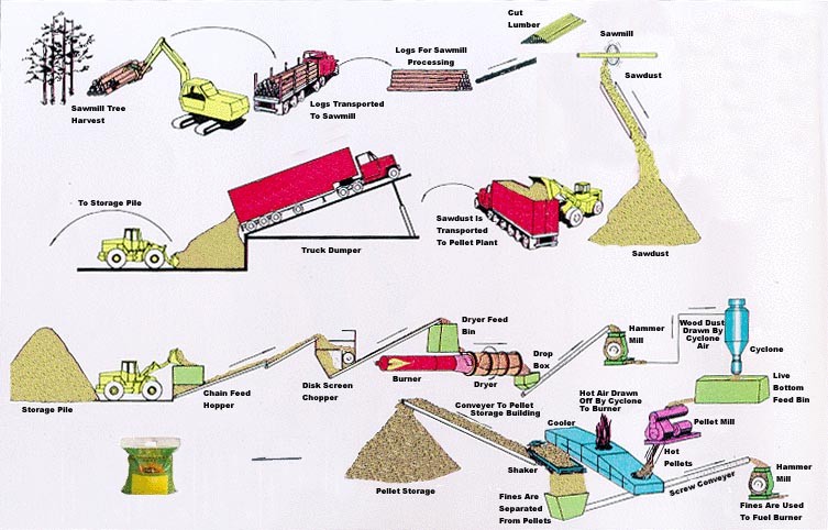
    [19] Energex. The Process of Making Energex Pellet Fuel. Available from: http://www.energex.com/common/images/process_large.jpg. (accessed August 15th., 2012).
    [20] International Organization for Standardization (2006) Environmental Management: Life Cycle Assessment : Principles and Framework. Geneva: ISO.
    [21] Natural Resources Canada (2009) Status of Energy Use in Canadian Wood Productions Sector. 978-1-100-52199-2. Ottawa: Natural Resources Canada.
    [22] Mani S (2005) A Systems Analysis of Biomass Densification Process. PhD thesis. Vancouver, Canada: University of British Columbia.
    [23] Food and Rural Affairs of Ontario (2010) Growing Greenhouse Vegetables in Ontario. Toronto, Canada, Queen's Printer for Ontario.
    [24] Bhat IK, Prakash R (2009) LCA of renewable energy for electricity generation systems-a review. Renew Sust Energ Rev 13: 1067-1073.
    [25] Hydro-Quebec (2010) Hydro-Quebec Production. 2011. Available from: http://www.hydroquebec.com/generation/.
    [26] Tremblay A, Varfalvy L, Roehm C, et al. (2004) The Issue of Greenhouse Gases from Hydroelectric Reservoirs: from Boreal to Tropical Regions. In proceddings of the United Nations Symposium on Hydropower and Sustainable Development, Beijing, China.
    [27] Fulton M, Kitasei S, Bluestein J (2011) Comparing Life-Cycle Greenhouse Gas Emissions from Natural Gas and Coal. Deutsche Bank Group.
    [28] Statistics Canada (2012a) Energy Statistics Handbook 57-601-XIE. Ottawa: Minister of Industry. Available from: http://www.statcan.gc.ca/pub/57-601-x/2012001/t188-eng.htm.
    [29] Sjølie HK, Solberg B (2011) Greenhouse gas emission impacts of use of Norwegian wood pellets: a sensitivity analysis. Environ Sci Policy 14: 1028-1040. doi: 10.1016/j.envsci.2011.07.011
    [30] Murphy F, Devlin G, McDonnell K (2015) Greenhouse gas and energy based life cycle analysis of products from the Irish wood processing industry. J Cleaner Prod 92: 134-141.
    [31] Statistics Canada (2012b) Greenhouse, Sod and Nursery Industries 2011. 22-202-XWE. Ottawa: Minister of Industry.
    [32] Argus (2011) Argus Biomass Market.
    [33] Wees D (2008) The Greenhouse Handbook. Montreal, Canada, McGill University.
    [34] Canakci M, Akinci I (2006) Energy Use Pattern Analyses of Greenhouse Vegetable Production. Energy 31: 1243-1256. doi: 10.1016/j.energy.2005.05.021
  • This article has been cited by:

    1. Ze Chen, Min Li, Hongxing Cui, Xipeng Wu, Fangmin Chen, Wei Li, Effects of kinesio taping therapy on gait and surface electromyography in stroke patients with hemiplegia, 2022, 13, 1664-042X, 10.3389/fphys.2022.1040278
    2. Runping Yuan, Congzhi Tang, Yong Jiang, Hongxing Wang, 2022, Effects of upper limb robot-assisted rehabilitation on motor function recovery and neuromuscular electrophysiological changes of stroke patients, 9781450395854, 73, 10.1145/3529261.3529274
    3. Yuqi LI, Guozhi HUANG, Pengcheng LU, Longlong HE, Wenhao HUANG, Chuhong HUANG, Qing ZENG, Effect of Rehabilitation Robot Combined with Upper Limb Rehabilitation Training on Hemiplegic Patients in Recovery Stage of Stroke, 2022, 32, 2096-0328, 111, 10.3724/SP.J.1329.2022.02004
    4. Le Wu, Xu Zhang, Xuan Zhang, Xiang Chen, Xun Chen, Metric learning for novel motion rejection in high-density myoelectric pattern recognition, 2021, 227, 09507051, 107165, 10.1016/j.knosys.2021.107165
    5. Dongdong Bu, Shuxiang Guo, Jin Guo, He Li, Hanze Wang, Low-Density sEMG-Based Pattern Recognition of Unrelated Movements Rejection for Wrist Joint Rehabilitation, 2023, 14, 2072-666X, 555, 10.3390/mi14030555
    6. Runping Yuan, Xu Qiao, Congzhi Tang, Ting Zhou, Wenli Chen, Ruyan Song, Yong Jiang, Jan D. Reinhardt, Hongxing Wang, Effects of Uni- vs. Bilateral Upper Limb Robot-Assisted Rehabilitation on Motor Function, Activities of Daily Living, and Electromyography in Hemiplegic Stroke: A Single-Blinded Three-Arm Randomized Controlled Trial, 2023, 12, 2077-0383, 2950, 10.3390/jcm12082950
    7. Beatriz Madroñero-Miguel, César Cuesta-García, Spanish consensus of occupational therapists on upper limb assessment tools in stroke, 2023, 86, 0308-0226, 648, 10.1177/03080226231175574
    8. Wenwen Lv, Kai Liu, Ping Zhou, Fei Huang, Zhiyuan Lu, Surface EMG analysis of weakness distribution in upper limb muscles post-stroke, 2023, 14, 1664-2295, 10.3389/fneur.2023.1135564
    9. Denise Bolonhezi Ribeiro, Larissa Gomes Sartori, María Verónica González Méndez, Roger Burgo de Souza, Daniel Prado Campos, Paulo Broniera Júnior, José J. A. Mendes Junior, Eddy Krueger, MES-FES Interface Enhances Quadriceps Muscle Response in Sitting Position in Incomplete Spinal Cord Injury: Pilot Study, 2024, 6, 2673-1592, 643, 10.3390/prosthesis6030045
    10. I Wayan Widhiada, Tjokorda Gde Tirta Nindhia, Made Adi Guna Dharma, I Dewa Gede Agung Eka Putra, Divyananda Japara, Kadek Yuma Kusuma Dewi, Anak Agung Gede Cahya Wedanta, I Komang Arimbawa, 2024, Development of Muscle Strength Scale Monitoring System for Stroke Patients Using Sensor AD8619-Based Surface Electromyography, 9798400717055, 155, 10.1145/3669754.3669778
  • Reader Comments
  • © 2016 the Author(s), licensee AIMS Press. This is an open access article distributed under the terms of the Creative Commons Attribution License (http://creativecommons.org/licenses/by/4.0)
通讯作者: 陈斌, bchen63@163.com
  • 1. 

    沈阳化工大学材料科学与工程学院 沈阳 110142

  1. 本站搜索
  2. 百度学术搜索
  3. 万方数据库搜索
  4. CNKI搜索

Metrics

Article views(6408) PDF downloads(1160) Cited by(1)

/

DownLoad:  Full-Size Img  PowerPoint
Return
Return

Catalog