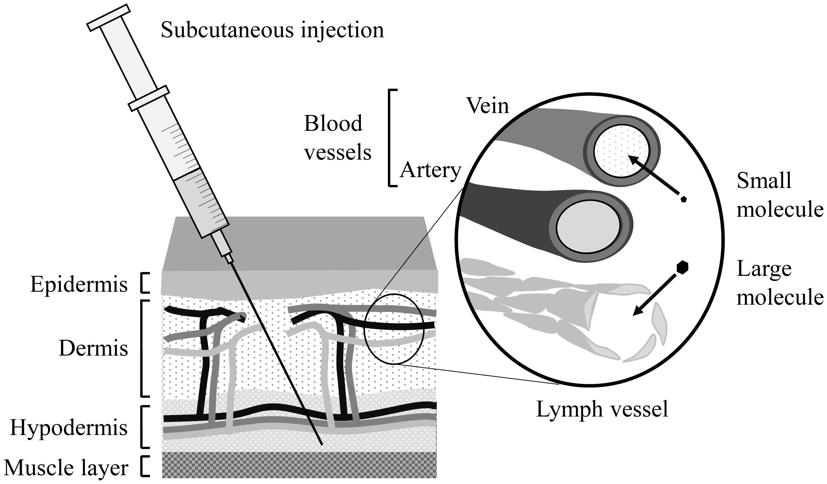
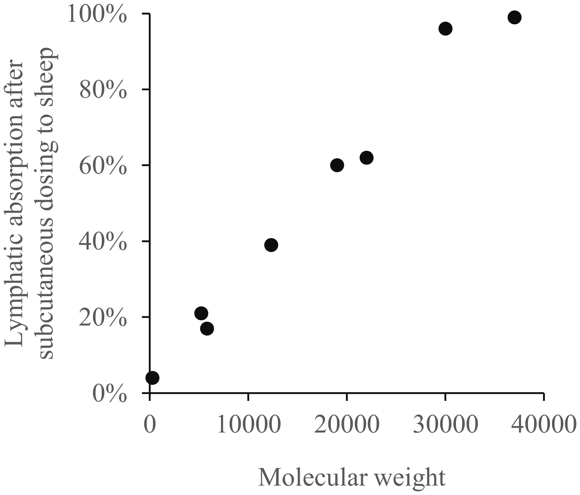
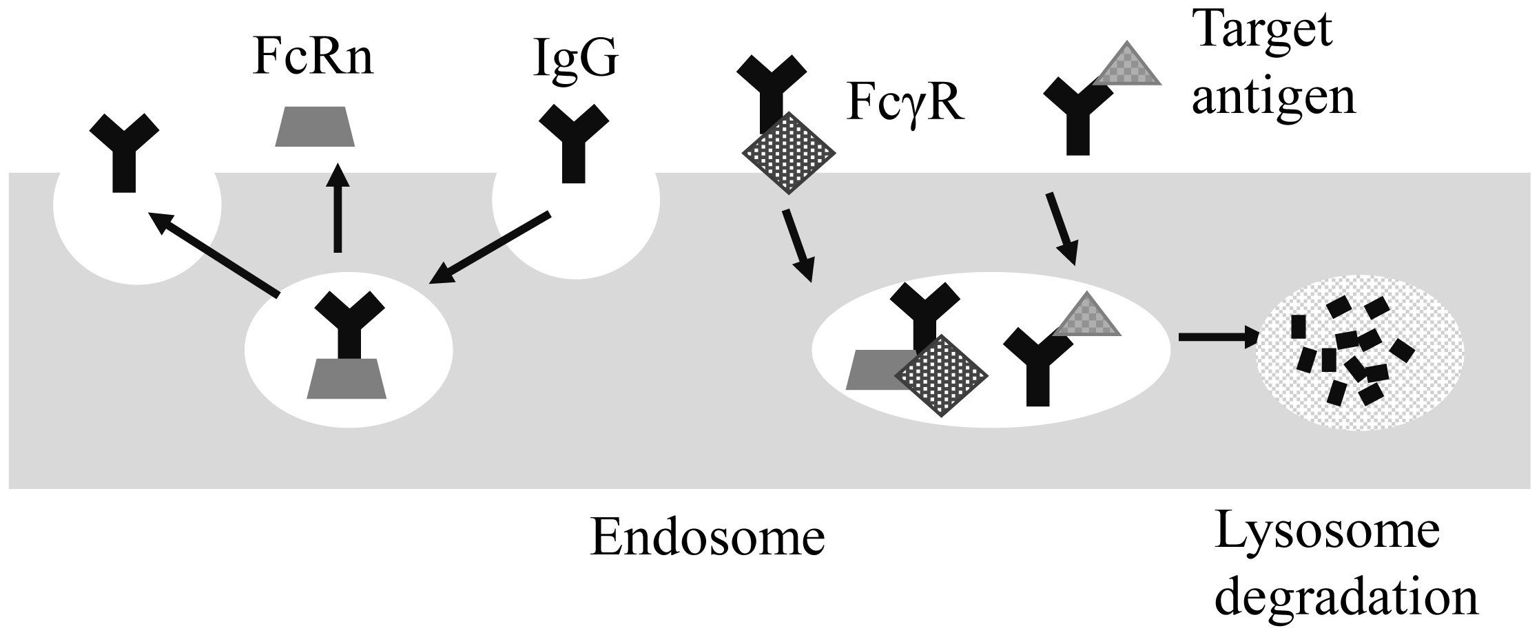
Subcutaneous (SC) sustained release is an important drug delivery system (DDS) for antibody/protein drugs because it reduces dosing frequency. This review discusses formulations and biophysical parameters that affect the pharmacokinetics (PK) of DDSs. For example, SC injectable microspheres and polymeric hydrogels, as well as intradermal microneedles, suppress denaturation in loading and burst release of drugs [growth hormone, interferon-α2b, bevacizumab, and single-chain antibody fragment (scFv)]. These DDSs significantly prolong half-life (t1/2) in plasma with low maximum concentration (Cmax) and low relative bioavailability after SC dosing to animals and/or humans. Formulation parameters, such as (1) drug loading amount, (2) drug diffusion in DDS, (3) interactions of drugs with polymers, and (4) microneedle design, likely contribute to their PK profiles. This review also discusses the effects of many biophysical parameters on PK, including (5) in vivo behavior of polymers (swelling, aggregation, dissolution, and accumulation), (6) drug interactions with extracellular matrix and hypodermis diffusion, (7) drug unfolding, (8) hypodermic concentration of drugs, inherent proteins, and cells, (9) drug absorption through lymphatic or blood vessels, (10) degradation of drugs/polymers by proteases/phagocytic cells, (11) FcRn-mediated recycling, (12) FcγR-mediated endocytosis, and (13) target-mediated drug clearance. For safe dosing, (14) skin's thickness/viscoelastic properties and variations and (15) skin's recovery are also important factors. Consideration of these effects will increase the developmental speed and success of many SC sustained-release DDSs of antibody/protein drugs.
Citation: Takayuki Yoshida, Hiroyuki Kojima. Subcutaneous sustained-release drug delivery system for antibodies and proteins[J]. AIMS Biophysics, 2025, 12(1): 69-100. doi: 10.3934/biophy.2025006
Subcutaneous (SC) sustained release is an important drug delivery system (DDS) for antibody/protein drugs because it reduces dosing frequency. This review discusses formulations and biophysical parameters that affect the pharmacokinetics (PK) of DDSs. For example, SC injectable microspheres and polymeric hydrogels, as well as intradermal microneedles, suppress denaturation in loading and burst release of drugs [growth hormone, interferon-α2b, bevacizumab, and single-chain antibody fragment (scFv)]. These DDSs significantly prolong half-life (t1/2) in plasma with low maximum concentration (Cmax) and low relative bioavailability after SC dosing to animals and/or humans. Formulation parameters, such as (1) drug loading amount, (2) drug diffusion in DDS, (3) interactions of drugs with polymers, and (4) microneedle design, likely contribute to their PK profiles. This review also discusses the effects of many biophysical parameters on PK, including (5) in vivo behavior of polymers (swelling, aggregation, dissolution, and accumulation), (6) drug interactions with extracellular matrix and hypodermis diffusion, (7) drug unfolding, (8) hypodermic concentration of drugs, inherent proteins, and cells, (9) drug absorption through lymphatic or blood vessels, (10) degradation of drugs/polymers by proteases/phagocytic cells, (11) FcRn-mediated recycling, (12) FcγR-mediated endocytosis, and (13) target-mediated drug clearance. For safe dosing, (14) skin's thickness/viscoelastic properties and variations and (15) skin's recovery are also important factors. Consideration of these effects will increase the developmental speed and success of many SC sustained-release DDSs of antibody/protein drugs.

| [1] | Martin KP, Grimaldi C, Grempler R, et al. (2023) Trends in industrialization of biotherapeutics: a survey of product characteristics of 89 antibody-based biotherapeutics. MAbs 15: 2191301. https://doi.org/10.1080/19420862.2023.2191301 |
| [2] | Shepard HM, Phillips GL, Thanos CD, et al. (2017) Developments in therapy with monoclonal antibodies and related proteins. Clin Med 17: 220-232. https://doi.org/10.7861/clinmedicine.17-3-220 |
| [3] | Lu RM, Hwang YC, Liu IJ, et al. (2020) Development of therapeutic antibodies for the treatment of diseases. J Biomed Sci 27: 1. https://doi.org/10.1186/s12929-019-0592-z |
| [4] | Zhou Y, Zhang Y, Chen Z, et al. (2024) Dynamic clinical success rates for drugs in the 21st century. medRxiv . https://doi.org/10.1101/2024.02.26.24303388 |
| [5] | Ovacik M, Lin K (2018) Tutorial on monoclonal antibody pharmacokinetics and its considerations in early development. Clin Transl Sci 11: 540-552. https://doi.org/10.1111/cts.12567 |
| [6] | Morales JO, Fathe KR, Brunaugh A, et al. (2017) Challenges and future prospects for the delivery of biologics: oral mucosal, pulmonary, and transdermal routes. AAPS J 19: 652-668. https://doi.org/10.1208/s12248-017-0054-z |
| [7] | Gill HS, Denson DD, Burris BA, et al. (2008) Effect of microneedle design on pain in human volunteers. Clin J Pain 24: 585-594. https://doi.org/10.1097/AJP.0b013e31816778f9 |
| [8] |
Parra A, Hernández C, Prieto-Pinto L (2023) Evaluation of the economic benefits, administration times, and patient preferences associated with the use of biotechnological drugs administered subcutaneously and intravenously in patients with cancer: a systematic review. Expert Rev Pharmacoecon Outcomes Res 23: 1017-1026. https://doi.org/10.1080/14737167.2023.2249232 
|
| [9] | Tomasini L, Ferrere M, Nicolas J (2024) Subcutaneous drug delivery from nanoscale systems. Nat Rev Bioeng 2: 501-520. https://doi.org/10.1038/s44222-024-00161-w |
| [10] |
Epstein RS (2021) Payer perspectives on intravenous versus subcutaneous administration of drugs. Clinicoecon Outcomes Res 13: 801-807. https://doi.org/10.2147/CEOR.S317687
|
| [11] |
Anderson KC, Landgren O, Arend RC, et al. (2019) Humanistic and economic impact of subcutaneous versus intravenous administration of oncology biologics. Future Oncol 15: 3267-3281. https://doi.org/10.2217/fon-2019-0368
|
| [12] | Cappuzzo1 F, Zvirbule Z, Korbenfeld EP, et al. (2024) 244mo primary results from imscin002: a study to evaluate patient (pt)- and healthcare professional (hcp)-reported preferences for atezolizumab (atezo) subcutaneous (sc) vs intravenous (iv) for the treatment of NSCLC. EMBO Open 9: 102706. https://doi.org/10.1016/j.esmoop.2024.102706 |
| [13] |
Knowles SP, Printz MA, Kang DW, et al. (2021) Safety of recombinant human hyaluronidase ph20 for subcutaneous drug delivery. Expert Opin Drug Deliv 18: 1673-1685. https://doi.org/10.1080/17425247.2021.1981286
|
| [14] |
Bittner B, Schmidt J (2024) Advancing subcutaneous dosing regimens for biotherapeutics: clinical strategies for expedited market access. BioDrugs 38: 23-46. https://doi.org/10.1007/s40259-023-00626-1
|
| [15] |
Leconet W, Liu H, Guo M, et al. (2018) Anti-PSMA/CD3 bispecific antibody delivery and antitumor activity using a polymeric depot formulation. Mol Cancer Ther 17: 1927-1940. https://doi.org/10.1158/1535-7163.MCT-17-1138
|
| [16] |
Kasse CM, Yu AC, Powell AE, et al. (2023) Subcutaneous delivery of an antibody against SARS-CoV-2 from a supramolecular hydrogel depot. Biomater Sci 11: 2065-2079. https://doi.org/10.1039/d2bm00819j
|
| [17] |
Van Beers MMC, Slooten C, Meulenaar J, et al. (2017) Micro-flow imaging as a quantitative tool to assess size and agglomeration of PLGA microparticles. Eur J Pharm Biopharm 117: 91-104. https://doi.org/10.1016/j.ejpb.2017.04.002
|
| [18] |
Abulateefeh SR (2023) Long-acting injectable PLGA/PLA depots for leuprolide acetate: successful translation from bench to clinic. Drug Deliv Transl Re 13: 520-530. https://doi.org/10.1007/s13346-022-01228-0
|
| [19] | Sali SR, Gondkar SB, Saudagar RB (2018) A review on: atrigel—the magical tool. Int J Curr Pharm Res 8: 48-54. https://doi.org/10.22159/ijcpr.2018v10i2.25890 |
| [20] |
Tornøe CW, Agersø H, Nielsen HA, et al. (2004) Population pharmacokinetic modeling of a subcutaneous depot for GnRH antagonist degarelix. Pharm Res 21: 574-584. https://doi.org/10.1023/b:pham.0000022403.60314.51
|
| [21] | Fatima H, Shukrullah S, Hussain H, et al. (2023) Utility of various drug delivery systems and their advantages and disadvantages. Nanotechnology for Drug Delivery and Pharmaceuticals . New York: Academic Press 235-258. https://doi.org/10.1016/B978-0-323-95325-2.00015-8 |
| [22] |
Hoffman AR, Biller BMK, Cook D, et al. (2005) Efficacy of a long-acting growth hormone (gh) preparation in patients with adult gh deficiency. J Clin Endocrinol Metab 90: 6431-6440. https://doi.org/10.1210/jc.2005-0928
|
| [23] |
McKay WF, Peckham SM, Badura JM (2007) A comprehensive clinical review of recombinant human bone morphogenetic protein-2 (INFUSE bone graft). Int Orthop 31: 729-734. https://doi.org/10.1007/s00264-007-0418-6
|
| [24] |
Chen Z, Kankala RK, Yang Z, et al. (2022) Antibody-based drug delivery systems for cancer therapy: mechanisms, challenges, and prospects. Theranostics 12: 3719-3746. https://doi.org/10.7150/thno.72594
|
| [25] |
Ojaimi YA, Blin T, Lamamy J, et al. (2022) Therapeutic antibodies—natural and pathological barriers and strategies to overcome them. Pharmacol Ther 233: 108022. https://doi.org/10.1016/j.pharmthera.2021.108022
|
| [26] |
Swartz MA, Fleury ME (2007) Interstitial flow and its effects in soft tissues. Annu Rev Biomed Eng 9: 229-256. https://doi.org/10.1146/annurev.bioeng.9.060906.151850
|
| [27] |
Stader F, Liu C, Derbalah A, et al. (2024) A physiologically based pharmacokinetic model relates the subcutaneous bioavailability of monoclonal antibodies to the saturation of FcRn-mediated recycling in injection-site-draining lymph nodes. Antibodies (Basel) 13: 70. https://doi.org/10.3390/antib13030070
|
| [28] |
Wu F, Bhansali SG, Law WC, et al. (2012) Fluorescence imaging of the lymph node uptake of proteins in mice after subcutaneous injection: molecular weight dependence. Pharm Res 29: 1843-1853. https://doi.org/10.1007/s11095-012-0708-6
|
| [29] |
Zhong X, Liu Y, Ardekani AM (2024) A compartment model for subcutaneous injection of monoclonal antibodies. Int J Pharm 650: 123687. https://doi.org/10.1016/j.ijpharm.2023.123687
|
| [30] |
Datta-Mannan A, Estwick S, Zhou C, et al. (2020) Influence of physiochemical properties on the subcutaneous absorption and bioavailability of monoclonal antibodies. MAbs 12: 1770028. https://doi.org/10.1080/19420862.2020.1770028
|
| [31] |
Mieczkowski CA (2023) The evolution of commercial antibody formulations. J Pharm Sci 112: 1801-1810. https://doi.org/10.1016/j.xphs.2023.03.026
|
| [32] |
Kinderman F, Yerby B, Jawa V, et al. (2019) Impact of precipitation of antibody therapeutics after subcutaneous injection on pharmacokinetics and immunogenicity. J Pharm Sci 108: 1953-1963. https://doi.org/10.1016/j.xphs.2019.01.015
|
| [33] |
Kijanka G, Bee JS, Bishop SM, et al. (2016) Fate of multimeric oligomers, submicron, and micron size aggregates of monoclonal antibodies upon subcutaneous injection in mice. J Pharm Sci 105: 1693-1704. https://doi.org/10.1016/j.xphs.2016.02.034
|
| [34] |
Filipe V, Que I, Carpenter JF, et al. (2014) In vivo fluorescence imaging of IgG1 aggregates after subcutaneous and intravenous injection in mice. Pharm Res 31: 216-227. https://doi.org/10.1007/s11095-013-1154-9
|
| [35] | Kijanka G, Prokopowicz M, Schellekens H, et al. (2014) Influence of aggregation and route of injection on the biodistribution of mouse serum albumin. Plos One 9: e85281. https://doi.org/10.1371/journal.pone.0085281 |
| [36] |
Wang W, Chen N, Shen X, et al. (2012) Lymphatic transport and catabolism of therapeutic proteins after subcutaneous administration to rats and dogs. Drug Metab Dispos 40: 952-962. https://doi.org/10.1124/dmd.111.043604
|
| [37] |
Thomas VA, Balthasar JP (2019) Understanding inter-individual variability in monoclonal antibody disposition. Antibodies (Basel) 8: 56. https://doi.org/10.3390/antib8040056
|
| [38] |
Richter WF, Bhansali SG, Morris ME (2012) Mechanistic determinants of biotherapeutics absorption following SC administration. AAPS J 14: 559-570. https://doi.org/10.1208/s12248-012-9367-0
|
| [39] |
Supersaxo A, Hein WR, Steffen H (1990) Effect of molecular weight on the lymphatic absorption of water-soluble compounds following subcutaneous administration. Pharm Res 7: 167-169. https://doi.org/10.1023/a:1015880819328
|
| [40] |
Yang TH, Cleland JL, Lam X, et al. (2000) Effect of zinc binding and precipitation on structures of recombinant human growth hormone and nerve growth factor. J Pharm Sci 89: 1480-1485. https://doi.org/10.1002/1520-6017(200011)89:11<1480::aid-jps10>3.0.co;2-m
|
| [41] |
Höybye C (2023) Comparing treatment with daily and long-acting growth hormone formulations in adults with growth hormone deficiency: challenging issues, benefits, and risks. Best Pract Res Clin Endocrinol Metab 37: 101788. https://doi.org/10.1016/j.beem.2023.101788
|
| [42] | Cai Y, Xu M, Yuan M, et al. (2014) Developments in human growth hormone preparations: sustained-release, prolonged half-life, novel injection devices, and alternative delivery routes. Int J Nanomedicine 9: 3527-3538. https://doi.org/10.2147/IJN.S63507 |
| [43] | FDA label, Eli Lilly and Company: Humatrope® somatropin (rDNA origin) for injection vials and cartridges (2005). Available from: https://www.accessdata.fda.gov/drugsatfda_docs/label/2006/019640s047,019640s052lbl.pdf |
| [44] |
Jordan F, Naylor A, Kelly CA, et al. (2010) Sustained release hGH microsphere formulation produced by a novel supercritical fluid technology: in vivo studies. J Control Release 141: 153-160. https://doi.org/10.1016/j.jconrel.2009.09.013
|
| [45] |
Tracy MA (1998) Development and scale-up of a microsphere protein delivery system. Biotechnol Prog 14: 108-115. https://doi.org/10.1021/bp9701271
|
| [46] |
Park K, Skidmore S, Hadar J, et al. (2019) Injectable, long-acting PLGA formulations: analyzing PLGA and understanding microparticle formation. J Control Release 304: 125-134. https://doi.org/10.1016/j.jconrel.2019.05.003
|
| [47] |
Oe Y, Kobayashi M, Yoshida T, et al. (2024) Injectable testosterone PLGA microsphere with different characteristics: effect of preparation method (paddle mixing versus microfluidic device). Pharm Dev Technol 29: 482-491. https://doi.org/10.1080/10837450.2024.2348580
|
| [48] |
Kojima R, Yoshida T, Tasaki H, et al. (2015) Release mechanisms of tacrolimus-loaded PLGA and PLA microspheres and immunosuppressive effects of the microspheres in a rat heart transplantation model. Int J Pharm 492: 20-27. https://doi.org/10.1016/j.ijpharm.2015.07.004
|
| [49] |
van de Weert M, Hoechstetter J, Hennink WE, et al. (2000) The effect of a water/organic solvent interface on the structural stability of lysozyme. J Control Release 68: 351-359. https://doi.org/10.1016/s0168-3659(00)00277-7
|
| [50] |
Su Y, Zhang B, Sun R, et al. (2021) PLGA-based biodegradable microspheres in drug delivery: recent advances in research and application. Drug Deliv 28: 1397-1418. https://doi.org/10.1080/10717544.2021.1938756
|
| [51] | FDA label, Genentech, Inc.: Nutropin Depot® somatropin (rDNA origin) for injectable suspension (1999). Available from: https://www.accessdata.fda.gov/drugsatfda_docs/label/2004/21075s008lbl.pdf |
| [52] |
Kemp SF, Fielder PJ, Attie KM, et al. (2004) Pharmacokinetic and pharmacodynamic characteristics of a long-acting growth hormone (GH) preparation (nutropin depot) in GH-deficient children. J Clin Endocrinol Metab 89: 3234-3240. https://doi.org/10.1210/jc.2003-030825
|
| [53] |
Shive MS, Anderson JM (1997) Biodegradation and biocompatibility of PLA and PLGA microspheres. Adv Drug Deliv Rev 28: 5-24. https://doi.org/10.1016/s0169-409x(97)00048-3
|
| [54] |
Zhang H, Yang Z, Wu D, et al. (2023) The effect of polymer blends on the in vitro release/degradation and pharmacokinetics of moxidectin-loaded PLGA microspheres. Int J Mol Sci 24: 14729. https://doi.org/10.3390/ijms241914729
|
| [55] |
Shah VR, Gupta PK (2018) Structural stability of recombinant human growth hormone (r-hGH) as a function of polymer surface properties. Pharm Res 35: 98. https://doi.org/10.1007/s11095-018-2372-y
|
| [56] |
Bosquillon C, Préat V, Vanbever R (2004) Pulmonary delivery of growth hormone using dry powders and visualization of its local fate in rats. J Control Release 96: 233-244. https://doi.org/10.1016/j.jconrel.2004.01.027
|
| [57] | Patton JS, McCabe JG, Hansen SE, et al. (1989) Absorption of human growth hormone from the rat lung. Biotechnol Ther 1: 213-228. |
| [58] |
Shive MS, Anderson JM (1997) Biodegradation and biocompatibility of PLA and PLGA microspheres. Adv Drug Deliv Rev 28: 5-24. https://doi.org/10.1016/s0169-409x(97)00048-3
|
| [59] | Ningrum RA (2014) Human interferon alpha-2b: a therapeutic protein for cancer treatment. Scientifica (Cairo) : 970315. https://doi.org/10.1155/2014/970315 |
| [60] |
Radwanski E, Perentesis G, Jacobs S, et al. (1987) Pharmacokinetics of interferon alpha-2b in healthy volunteers. J Clin Pharmacol 27: 432-435. https://doi.org/10.1002/j.1552-4604.1987.tb03044.x
|
| [61] |
Li Z, Li L, Liu Y, et al. (2011) Development of interferon alpha-2b microspheres with constant release. Int J Pharm 410: 48-53. https://doi.org/10.1016/j.ijpharm.2011.03.016
|
| [62] |
Chan Y-P, Meyrueix R, Kravtzoff R, et al. (2007) Review on Medusa®: a polymer-based sustained release technology for protein and peptide drugs. Expert Opin Drug Deliv 4: 441-451. https://doi.org/10.1517/17425247.4.4.441
|
| [63] |
Trépo C, Meyrueix R, Maynard M, et al. (2006) Novel sustained release formulation of IFNα-2b improves tolerability and demonstrates potent viral load reduction in a phase I/II HCV clinical trial. J Clin Virol 36: S24. https://doi.org/10.1016/S1386-6532(06)80081-8
|
| [64] | Bonnet-Gonnet C, Chognot D, Soula O, et al. (2014) Pharmaceutical formulations for the prolonged release of active principle(s), and their applications, especially therapeutic applications. US Patent : 8679540 B2. |
| [65] |
Hill CP, Osslund TD, Eisenberg D (1993) The structure of granulocyte-colony-stimulating factor and its relationship to other growth factors. Proc Natl Acad Sci USA 90: 5167-5171. https://doi.org/10.1073/pnas.90.11.5167
|
| [66] |
Nagabhushan TL, Reichert P, Walter MR, et al. (2011) Type I interferon structures: possible scaffolds for the interferon-alpha receptor complex. Can J Chem 80: 1166-1173. https://doi.org/10.1139/v02-158
|
| [67] |
Chino M, Maglio O, Nastri F, et al. (2015) Artificial diiron enzymes with a de novo designed four-helix bundle structure. Eur J Inorg Chem 21: 3371-3390. https://doi.org/10.1002/ejic.201500470
|
| [68] |
Schaefer MH, Wanker EE, Andrade-Navarro MA (2012) Evolution and function of CAG/polyglutamine repeats in protein-protein interaction networks. Nucleic Acids Res 40: 4273-4287. https://doi.org/10.1093/nar/gks011
|
| [69] |
Jakubek RS, Workman RJ, White SE, et al. (2019) Polyglutamine solution-state structural propensity is repeat length dependent. J Phys Chem B 123: 4193-4203. https://doi.org/10.1021/acs.jpcb.9b01433
|
| [70] |
Rathod S, Bahadur P, Tiwari S (2021) Nanocarriers based on vitamin E-TPGS: Design principle and molecular insights into improving the efficacy of anticancer drugs. Int J Pharm 592: 120045. https://doi.org/10.1016/j.ijpharm.2020.120045
|
| [71] |
Ellmerer M, Schaupp L, Brunner GA, et al. (2000) Measurement of interstitial albumin in human skeletal muscle and adipose tissue by open-flow microperfusion. Am J Physiol Endocrinol Metab 278: E352-356. https://doi.org/10.1152/ajpendo.2000.278.2.E352
|
| [72] |
Kaja S, Hilgenberg JD, Everett E, et al. (2011) Effects of dilution and prolonged storage with preservative in a polyethylene container on Bevacizumab (Avastin™) for topical delivery as a nasal spray in anti-hereditary hemorrhagic telangiectasia and related therapies. Hum Antibodies 20: 95-101. https://doi.org/10.3233/HAB-2011-0244
|
| [73] |
Elebiyo TC, Rotimi D, Evbuomwan IO, et al. (2022) Reassessing vascular endothelial growth factor (VEGF) in anti-angiogenic cancer therapy. Cancer Treat Res Commun 32: 100620. https://doi.org/10.1016/j.ctarc.2022.100620
|
| [74] |
Lu JF, Bruno R, Eppler S, et al. (2008) Clinical pharmacokinetics of bevacizumab in patients with solid tumors. Cancer Chemoth Pharm 62: 779-786. https://doi.org/10.1007/s00280-007-0664-8
|
| [75] |
Lee ALZ, Ng VWL, Gao S, et al. (2015) Injectable biodegradable hydrogels from vitamin D-functionalized polycarbonates for the delivery of avastin with enhanced therapeutic efficiency against metastatic colorectal cancer. Biomacromolecules 16: 465-475. https://doi.org/10.1021/bm5015206
|
| [76] |
Fletcher NA, Krebs MD (2018) Sustained delivery of anti-VEGF from injectable hydrogel systems provides a prolonged decrease of endothelial cell proliferation and angiogenesis in vitro. RSC Adv 8: 8999-9005. https://doi.org/10.1039/c7ra13014g
|
| [77] |
Courtenay AJ, McCrudden MTC, McAvoy KJ, et al. (2018) Microneedle-mediated transdermal delivery of bevacizumab. Mol Pharm 15: 3545-3556. https://doi.org/10.1021/acs.molpharmaceut.8b00544
|
| [78] |
Huynh V, Wylie RG (2019) Displacement affinity release of antibodies from injectable hydrogels. ACS Appl Mater Interfaces 11: 30648-30660. https://doi.org/10.1021/acsami.9b12572
|
| [79] |
Gregoritza M, Messmann V, Abstiens K, et al. (2017) Controlled antibody release from degradable thermoresponsive hydrogels cross-linked by Diels-Alder chemistry. Biomacromolecules 18: 2410-2418. https://doi.org/10.1021/acs.biomac.7b00587
|
| [80] |
Huynh V, Wylie RG (2018) Competitive affinity release for long-term delivery of antibodies from hydrogels. Angew Chem Int Ed Engl 57: 3406-3410. https://doi.org/10.1002/anie.201713428
|
| [81] |
Lin YS, Nguyen C, Mendoza JL, et al. (1999) Preclinical pharmacokinetics, interspecies scaling, and tissue distribution of a humanized monoclonal antibody against vascular endothelial growth factor. J Pharmacol Exp Ther 288: 371-378.
|
| [82] |
Lee ALZ, Ng VWL, Poon GL, et al. (2015) Co-delivery of antiviral and antifungal therapeutics for the treatment of sexually transmitted infections using a moldable, supramolecular hydrogel. Adv Healthc Mater 4: 385-394. https://doi.org/10.1002/adhm.201400340
|
| [83] | Ghosh I, Gutka H, Krause ME, et al. (2023) A systematic review of commercial high concentration antibody drug products approved in the US: formulation composition, dosage form design and primary packaging considerations. MAbs 15: 2205540. https://doi.org/10.1080/19420862.2023.2205540 |
| [84] |
Yang C, Lee A, Gao S, et al. (2019) Hydrogels with prolonged release of therapeutic antibody: Block junction chemistry modification of ‘ABA’ copolymers provides superior anticancer efficacy. J Control Release 293: 193-200. https://doi.org/10.1016/j.jconrel.2018.11.026
|
| [85] |
Kyriakides TR, Kim HJ, Zheng C, et al. (2022) Foreign body response to synthetic polymer biomaterials and the role of adaptive immunity. Biomed Mater 17: 022007. https://doi.org/10.1088/1748-605X/ac5574
|
| [86] |
Challa DK, Wang X, Montoyo HP, et al. (2019) Neonatal Fc receptor expression in macrophages is indispensable for IgG homeostasis. MAbs 11: 848-860. https://doi.org/10.1080/19420862.2019.1602459
|
| [87] |
Stader F, Liu C, Derbalah A, et al. (2024) A physiologically based pharmacokinetic model relates the subcutaneous bioavailability of monoclonal antibodies to the saturation of FcRn-mediated recycling in injection-site-draining lymph nodes. Antibodies (Basel) 13: 70. https://doi.org/10.3390/antib13030070
|
| [88] | Davis JD, Padros MB, Conrado DJ, et al. (2024) Subcutaneous administration of monoclonal antibodies: pharmacology, delivery, immunogenicity, and learnings from applications to clinical development. Clin Pharmacol Ther 115: 422-439. https://doi.org/10.1002/cpt.3150 |
| [89] | Mould DR, Baumann A, Kuhlmann J, et al. (2007) Population pharmacokinetics-pharmacodynamics of alemtuzumab (Campath) in patients with chronic lymphocytic leukaemia and its link to treatment response. Br J Clin Pharmacol 64: 278-291. https://doi.org/10.1111/j.1365-2125.2007.02914.x |
| [90] | Gibbs JP, Doshi S, Kuchimanchi M, et al. (2017) Impact of target-mediated elimination on the dose and regimen of evolocumab, a human monoclonal antibody against proprotein convertase subtilisin/kexin type 9 (PCSK9). J Clin Pharmacol 57: 616-626. https://doi.org/10.1002/jcph.840 |
| [91] |
Rudnick SI, Lou J, Shaller CC, et al. (2011) Influence of affinity and antigen internalization on the uptake and penetration of anti-HER2 antibodies in solid tumors. Cancer Res 71: 2250-2259. https://doi.org/10.1158/0008-5472.CAN-10-2277
|
| [92] |
Finley SD, Dhar M, Popel AS (2013) Compartment model predicts VEGF secretion and investigates the effects of VEGF trap in tumor-bearing mice. Front Oncol 3: 196. https://doi.org/10.3389/fonc.2013.00196
|
| [93] |
Ng CM, Fielder PJ, Jin J, et al. (2016) Mechanism-based competitive binding model to investigate the effect of neonatal Fc receptor binding affinity on the pharmacokinetic of humanized anti-VEGF monoclonal IgG1 antibody in cynomolgus monkey. AAPS J 18: 948-959. https://doi.org/10.1208/s12248-016-9911-4
|
| [94] |
Keyes KA, Mann L, Sherman M, et al. (2004) LY317615 decreases plasma VEGF levels in human tumor xenograft-bearing mice. Cancer Chemother Pharmacol 53: 133-140. https://doi.org/10.1007/s00280-003-0713-x
|
| [95] |
van Bueren JJL, Bleeker WK, Bøgh HO, et al. (2006) Effect of target dynamics on pharmacokinetics of a novel therapeutic antibody against the epidermal growth factor receptor: implications for the mechanisms of action. Cancer Res 66: 7630-7638. https://doi.org/10.1158/0008-5472.CAN-05-4010
|
| [96] |
Schneider EL, Hearn BR, Pfaff SJ, et al. (2016) Approach for half-Life extension of small antibody fragments that does not affect tissue uptake. Bioconjug Chem 27: 2534-2539. https://doi.org/10.1021/acs.bioconjchem.6b00469
|
| [97] |
Ottiger M, Thiel MA, Feige U, et al. (2009) Efficient intraocular penetration of topical anti-TNF-alpha single-chain antibody (ESBA105) to anterior and posterior segment without penetration enhancer. Invest Ophthalmol Vis Sci 50: 779-786. https://doi.org/10.1167/iovs.08-2372
|
| [98] |
Muñoz-López P, Ribas-Aparicio RM, Becerra-Báez EI, et al. (2022) Single-chain fragment variable: recent progress in cancer diagnosis and therapy. Cancers (Basel) 14: 4206. https://doi.org/10.3390/cancers14174206
|
| [99] |
Furrer E, Berdugo M, Stella C, et al. (2009) Pharmacokinetics and posterior segment biodistribution of ESBA105, an anti-TNF-alpha single-chain antibody, upon topical administration to the rabbit eye. Invest Ophthalmol Vis Sci 50: 771-778. https://doi.org/10.1167/iovs.08-2370
|
| [100] |
Li Z, Krippendorff BF, Sharma S, et al. (2016) Influence of molecular size on tissue distribution of antibody fragments. mAbs 8: 113-119. https://doi.org/10.1080/19420862.2015.1111497
|
| [101] |
Knowles SM, Wu AM (2012) Advances in immuno-positron emission tomography: antibodies for molecular imaging in oncology. J Clin Oncol 30: 3884-3892. https://doi.org/10.1200/JCO.2012.42.4887
|
| [102] |
Sakai T, Matsunaga T, Yamamoto Y, et al. (2008) Design and fabrication of a high-strength hydrogel with ideally homogeneous network structure from tetrahedron-like macromonomers. Macromolecules 41: 5379-5384. https://doi.org/10.1021/ma800476x
|
| [103] |
Schneider EL, Henise J, Reid R, et al. (2016) Hydrogel drug delivery system using self-cleaving covalent linkers for once-a-week administration of exenatide. Bioconjug Chem 27: 1210-1215. https://doi.org/10.1021/acs.bioconjchem.5b00690
|
| [104] |
Santi DV, Schneider EL, Reid R, et al. (2012) Predictable and tunable half-life extension of therapeutic agents by controlled chemical release from macromolecular conjugates. Proc Natl Acad Sci U S A 109: 6211-6216. https://doi.org/10.1073/pnas.1117147109
|
| [105] |
Santi DV, Schneider EL, Ashley GW (2014) Macromolecular prodrug that provides the irinotecan (CPT-11) active-metabolite SN-38 with ultralong half-life, low C(max), and low glucuronide formation. J Med Chem 57: 2303-2314. https://doi.org/10.1021/jm401644v
|
| [106] |
Deb T, Tu J, Franzini RM (2021) Mechanisms and substituent effects of metal-free bioorthogonal reactions. Chem Rev 121: 6850-6914. https://doi.org/10.1021/acs.chemrev.0c01013
|
| [107] |
Klein G, Reymond JL (1998) An enantioselective fluorimetric assay for alcohol dehydrogenases using albumin-catalyzed beta-elimination of umbelliferone. Bioorg Med Chem Lett 8: 1113-1116. https://doi.org/10.1016/s0960-894x(98)00165-6
|
| [108] |
Tu J, Xu M, Parvez S, et al. (2018) Bioorthogonal removal of 3-isocyanopropyl groups enables the controlled release of fluorophores and drugs in vivo. J Am Chem Soc 140: 8410-8414. https://doi.org/10.1021/jacs.8b05093
|
| [109] |
Roller SG, Dieckhaus CM, Santos WL, et al. (2002) Interaction between human serum albumin and the felbamate metabolites 4-hydroxy-5-phenyl-
|
| [110] |
Xu M, Deb T, Tu J, et al. (2019) Tuning isonitrile/tetrazine chemistry for accelerated deprotection and formation of stable conjugates. J Org Chem 84: 15520-15529. https://doi.org/10.1021/acs.joc.9b02522
|
| [111] |
Sakai T, Fujiyabu T (2020) Control over swelling of injectable gel. Physics of Polymer Gels . Weinheim: Wiley-VCH 261-276. https://doi.org/10.1002/9783527346547.ch17
|
| [112] |
Li Z, Yu X, Li Y, et al. (2021) A two-pore physiologically based pharmacokinetic model to predict subcutaneously administered different-size antibody/antibody fragments. AAPS J 23: 62. https://doi.org/10.1208/s12248-021-00588-8
|
| [113] |
Richter WF, Christianson GJ, Frances N, et al. (2018) Hematopoietic cells as site of first-pass catabolism after subcutaneous dosing and contributors to systemic clearance of a monoclonal antibody in mice. mAbs 10: 803-813. https://doi.org/10.1080/19420862.2018.1458808
|
| [114] |
Hangasky JA, Chen W, Dubois SP, et al. (2022) A very long-acting IL-15: implications for the immunotherapy of cancer. J Immunother Cancer 10: e004104. https://doi.org/10.1136/jitc-2021-004104
|
| [115] |
Kirkby M, Hutton ARJ, Donnelly RF (2020) Microneedle mediated transdermal delivery of protein, peptide and antibody based therapeutics: current status and future considerations. Pharm Res 37: 117. https://doi.org/10.1007/s11095-020-02844-6
|
| [116] |
Zhao J, Xu G, Yao X, et al. (2022) Microneedle-based insulin transdermal delivery system: current status and translation challenges. Drug Deliv Transl Res 12: 2403-2427. https://doi.org/10.1007/s13346-021-01077-3
|
| [117] |
Zhang J, Li H, Albakr L, et al. (2023) Microneedle-enabled therapeutics delivery and biosensing in clinical trials. J Control Release 360: 687-704. https://doi.org/10.1016/j.jconrel.2023.07.023
|
| [118] |
McCrudden MTC, Alkilani AZ, McCrudden CM, et al. (2014) Design and physicochemical characterisation of novel dissolving polymeric microneedle arrays for transdermal delivery of high dose, low molecular weight drugs. J Control Release 180: 71-80. https://doi.org/10.1016/j.jconrel.2014.02.007
|
| [119] |
Duarah S, Sharma M, Wen J (2019) Recent advances in microneedle-based drug delivery: Special emphasis on its use in paediatric population. Eur J Pharm Biopharm 136: 48-69. https://doi.org/10.1016/j.ejpb.2019.01.005
|
| [120] |
Kashaninejad N, Munaz A, Moghadas H, et al. (2021) Microneedle arrays for sampling and sensing skin interstitial fluid. Chemosensors 9: 83. https://doi.org/10.3390/chemosensors9040083
|
| [121] |
Olatunji O, Das DB, Garland MJ, et al. (2013) Influence of array interspacing on the force required for successful microneedle skin penetration: theoretical and practical approaches. J Pharm Sci 102: 1209-1221. https://doi.org/10.1002/jps.23439
|
| [122] |
Pawlaczyk M, Lelonkiewicz M, Wieczorowski M (2013) Age-dependent biomechanical properties of the skin. Postepy Dermatol Alergol 30: 302-306. https://doi.org/10.5114/pdia.2013.38359
|
| [123] |
Sandby-Møller J, Poulsen T, Wulf HC (2003) Epidermal thickness at different body sites: relationship to age, gender, pigmentation, blood content, skin type and smoking habits. Acta Derm Venereol 83: 410-413. https://doi.org/10.1080/00015550310015419
|
| [124] |
Courtenay AJ, McCrudden MTC, McAvoy KJ, et al. (2018) Microneedle-mediated transdermal delivery of bevacizumab. Mol Pharm 15: 3545-3556. https://doi.org/10.1021/acs.molpharmaceut.8b00544
|
| [125] |
Amodwala S, Kumar P, Thakkar HP (2017) Statistically optimized fast dissolving microneedle transdermal patch of meloxicam: a patient friendly approach to manage arthritis. Eur J Pharm Sci 104: 114-123. https://doi.org/10.1016/j.ejps.2017.04.001
|
| [126] |
Hutton ARJ, Kirkby M, Bogaert TV, et al. (2024) Transdermal administration of nanobody molecules using hydrogel-forming microarray patch technology: a unique delivery approach. Macromol Mater Eng 309: 2400029. https://doi.org/10.1002/mame.202400029
|
| [127] |
Hirobe S, Susai R, Takeuchi H, et al. (2021) Characteristics of immune induction by transcutaneous vaccination using dissolving microneedle patches in mice. Int J Pharm 601: 120563. https://doi.org/10.1016/j.ijpharm.2021.120563
|
| [128] |
Kalluri H, Banga AK (2011) Formation and closure of microchannels in skin following microporation. Pharm Res 28: 82-94. https://doi.org/10.1007/s11095-010-0122-x
|
| [129] |
Jung EC, Maibach HI (2015) Animal models for percutaneous absorption. J Appl Toxicol 35: 1-10. https://doi.org/10.1002/jat.3004
|
| [130] |
Capt A, Luzy AP, Esdaile D, et al. (2007) Comparison of the human skin grafted onto nude mouse model with in vivo and in vitro models in the prediction of percutaneous penetration of three lipophilic pesticides. Regul Toxicol Pharmacol 47: 274-287. https://doi.org/10.1016/j.yrtph.2006.11.008
|
| [131] |
Scott RC, Dugard PH, Doss AW (1986) Permeability of abnormal rat skin. J Invest Dermatol 86: 201-207. https://doi.org/10.1111/1523-1747.ep12284280
|
| [132] |
Haq MI, Smith E, John DN, et al. (2009) Clinical administration of microneedles: skin puncture, pain and sensation. Biomed Microdevices 11: 35-47. https://doi.org/10.1007/s10544-008-9208-1
|
| [133] |
Al-Kasasbeh R, Brady AJ, Courtenay AJ, et al. (2020) Evaluation of the clinical impact of repeat application of hydrogel-forming microneedle array patches. Drug Deliv Transl Res 10: 690-705. https://doi.org/10.1007/s13346-020-00727-2
|

Figures(6) / Tables(9)

Takayuki Yoshida, Hiroyuki Kojima. Subcutaneous sustained-release drug delivery system for antibodies and proteins[J]. AIMS Biophysics, 2025, 12(1): 69-100. doi: 10.3934/biophy.2025006


 DownLoad: