Multi-class EEG signal classification with statistical binary pattern synergic network for schizophrenia severity diagnosis

Dr. P. Esther Rani; B.V.V.S.R.K.K. Pavan; Dr. P. Esther Rani; B.V.V.S.R.K.K. Pavan

doi:10.3934/biophy.2023021

AIMS Biophysics

2023, Volume 10, Issue 3: 347-371. doi: 10.3934/biophy.2023021

Previous Article Next Article

Research article

Multi-class EEG signal classification with statistical binary pattern synergic network for schizophrenia severity diagnosis

Dr. P. Esther Rani ¹,
B.V.V.S.R.K.K. Pavan ^{2
,
,}

1.
Professor in ECE Department, Vel Tech Rangarajan Dr. Sagunthala R & D Institute of Science and Technology, 4000 Feet Outer Ring Road, Avadi, Chennai 600062, Tamil Nadu, India
2.
Research Scholar, VelTech Rangarajan Dr. Sagunthala R & D Institute of Science and Technology 4000 Feet Outer Ring Road, Avadi, Chennai-600062, Tamil Nadu, India

Received: 04 April 2023 Revised: 23 July 2023 Accepted: 25 July 2023 Published: 20 September 2023

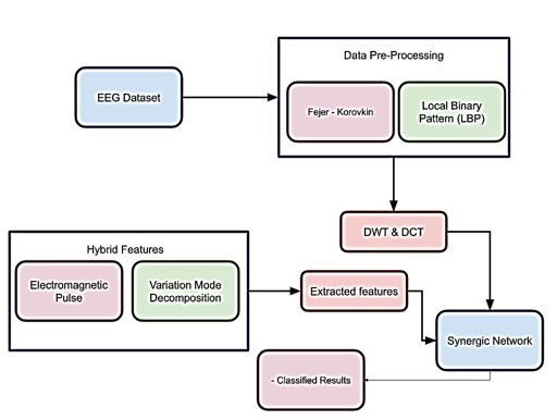
Electroencephalography (EEG) is a widely used medical procedure that helps to identify abnormalities in brain wave patterns and measures the electrical activity of the brain. The EEG signal comprises different features that need to be distinguished based on a specified property to exhibit recognizable measures and functional components that are then used to evaluate the pattern in the EEG signal. Through extraction, feature loss is minimized with the embedded signal information. Additionally, resources are minimized to compute the vast range of data accurately. It is necessary to minimize the information processing cost and implementation complexity to improve the information compression. Currently, different methods are being implemented for feature extraction in the EEG signal. The existing methods are subjected to different detection schemes that effectively stimulate the brain signal with the interface for medical rehabilitation and diagnosis. Schizophrenia is a mental disorder that affects the individual's reality abnormally. This paper proposes a statistical local binary pattern (SLBP) technique for feature extraction in EEG signals. The proposed SLBP model uses statistical features to compute EEG signal characteristics. Using Local Binary Pattern with proposed SLBP model texture based on a labeling signal with an estimation of the neighborhood in signal with binary search operation. The classification is performed for the earlier-prediction shizophrenia stage, either mild or severe. The analysis is performed considering three classes, i.e., normal, mild, and severe. The simulation results show that the proposed SLBP model achieved a classification accuracy of 98%, which is ~12% higher than the state-of-the-art methods.
- electroencephalogram,
- statistical features,
- local binary pattern,
- classification,
- synergic network
Citation: Dr. P. Esther Rani, B.V.V.S.R.K.K. Pavan. Multi-class EEG signal classification with statistical binary pattern synergic network for schizophrenia severity diagnosis[J]. AIMS Biophysics, 2023, 10(3): 347-371. doi: 10.3934/biophy.2023021

Related Papers:

Abstract

Electroencephalography (EEG) is a widely used medical procedure that helps to identify abnormalities in brain wave patterns and measures the electrical activity of the brain. The EEG signal comprises different features that need to be distinguished based on a specified property to exhibit recognizable measures and functional components that are then used to evaluate the pattern in the EEG signal. Through extraction, feature loss is minimized with the embedded signal information. Additionally, resources are minimized to compute the vast range of data accurately. It is necessary to minimize the information processing cost and implementation complexity to improve the information compression. Currently, different methods are being implemented for feature extraction in the EEG signal. The existing methods are subjected to different detection schemes that effectively stimulate the brain signal with the interface for medical rehabilitation and diagnosis. Schizophrenia is a mental disorder that affects the individual's reality abnormally. This paper proposes a statistical local binary pattern (SLBP) technique for feature extraction in EEG signals. The proposed SLBP model uses statistical features to compute EEG signal characteristics. Using Local Binary Pattern with proposed SLBP model texture based on a labeling signal with an estimation of the neighborhood in signal with binary search operation. The classification is performed for the earlier-prediction shizophrenia stage, either mild or severe. The analysis is performed considering three classes, i.e., normal, mild, and severe. The simulation results show that the proposed SLBP model achieved a classification accuracy of 98%, which is ~12% higher than the state-of-the-art methods.

References

[1]	Pahuja SK, Veer K (2022) Recent approaches on classification and feature extraction of EEG signal: a review. Robotica 40: 77–101. https://doi.org/10.1017/S0263574721000382 doi: 10.1017/S0263574721000382
[2]	Wang J, Wang M (2021) Review of the emotional feature extraction and classification using EEG signals. Cogn Robot 1: 29–40. https://doi.org/10.1016/j.cogr.2021.04.001 doi: 10.1016/j.cogr.2021.04.001
[3]	Li MA, Han JF, Yang JF (2021) Automatic feature extraction and fusion recognition of motor imagery EEG using multilevel multiscale CNN. Med Biol Eng Comput 59: 2037–2050. https://doi.org/10.1007/s11517-021-02396-w doi: 10.1007/s11517-021-02396-w
[4]	Baygin M, Dogan S, Tuncer T, et al. (2021) Automated ASD detection using hybrid deep lightweight features extracted from EEG signals. Comput Biol Med 134: 104548. https://doi.org/10.1016/j.compbiomed.2021.104548 doi: 10.1016/j.compbiomed.2021.104548
[5]	Zheng X, Liu X, Zhang Y, et al. (2021) A portable HCI system‐oriented EEG feature extraction and channel selection for emotion recognition. Int J Intell Syst 36: 152–176. https://doi.org/10.1002/int.22295 doi: 10.1002/int.22295
[6]	Tuncer T, Dogan S, Subasi A (2022) LEDPatNet19: Automated emotion recognition model based on nonlinear LED pattern feature extraction function using EEG signals. Cogn Neurodynamics 16: 779–790. https://doi.org/10.1007/s11571-021-09748-0 doi: 10.1007/s11571-021-09748-0
[7]	Suzuki K, Laohakangvalvit T, Matsubara R, et al. (2021) Constructing an emotion estimation model based on EEG/HRV indexes using feature extraction and feature selection algorithms. Sensors 21: 2910. https://doi.org/10.3390/s21092910 doi: 10.3390/s21092910
[8]	Tuncer T, Dogan S, Subasi A (2021) EEG-based driving fatigue detection using multilevel feature extraction and iterative hybrid feature selection. Biomed Signal Proces 68: 102591. https://doi.org/10.1016/j.bspc.2021.102591 doi: 10.1016/j.bspc.2021.102591
[9]	Woodbright M, Verma B, Haidar A (2021) Autonomous deep feature extraction based method for epileptic EEG brain seizure classification. Neurocomputing 444: 30–37. https://doi.org/10.1016/j.neucom.2021.02.052 doi: 10.1016/j.neucom.2021.02.052
[10]	Ein Shoka AA, Alkinani MH, El-Sherbeny AS, et al. (2021) Automated seizure diagnosis system based on feature extraction and channel selection using EEG signals. Brain Inform 8: 1–16. https://doi.org/10.1186%2Fs40708-021-00123-7
[11]	Albaqami H, Hassan GM, Subasi A, et al. (2021) Automatic detection of abnormal EEG signals using wavelet feature extraction and gradient boosting decision tree. Biomed Signal Proces 70: 102957. https://doi.org/10.1016/j.bspc.2021.102957 doi: 10.1016/j.bspc.2021.102957
[12]	Grossi E, Valbusa G, Buscema M (2021) Detection of an autism EEG signature from only two EEG channels through features extraction and advanced machine learning analysis. Clin EEG Neurosci 52: 330–337. https://doi.org/10.1177/1550059420982424 doi: 10.1177/1550059420982424
[13]	Deng X, Zhu J, Yang S (202) SFE-Net: EEG-based emotion recognition with symmetrical spatial feature extraction. In Proceedings of the 29th ACM International Conference on Multimedia, 2391–2400. https://doi.org/10.48550/arXiv.2104.06308
[14]	Kumar TR, Mahalaxmi U, Ramakrishna MM, et al. (2023) Optimization enabled deep residual neural network for motor signalry EEG signal classification. Biomed Signal Proces 80: 104317. https://doi.org/10.1016/j.bspc.2022.104317
[15]	de Paula PO, da Silva Costa TB, de Faissol Attux RR, et al. (2023) Classification of signal encoded SSVEP-based EEG signals using convolutional neural networks. Expert Syst Appl 214: 119096. https://doi.org/10.1016/j.eswa.2022.119096 doi: 10.1016/j.eswa.2022.119096
[16]	Fei SW, Chu YB (2022) A novel classification strategy of motor signalry EEG signals utilizing WT-PSR-SVD-based MTSVM. Expert Syst Appl 199: 116901. https://doi.org/10.1016/j.artmed.2019.101787 doi: 10.1016/j.artmed.2019.101787
[17]	Al-Salman W, Li Y, Oudah AY, et al. (2022) Sleep stage classification in EEG signals using the clustering approach based probability distribution features coupled with classification algorithms. Neurosci Res 188: 51–67. https://doi.org/10.1016/j.neures.2022.09.009 doi: 10.1016/j.neures.2022.09.009
[18]	Ma W, Xue H, Sun X, et al. (2022) A novel multi-branch hybrid neural network for motor signalry EEG signal classification. Biomed Signal Proces 77: 103718. https://doi.org/10.1016/j.bspc.2022.103718 doi: 10.1016/j.bspc.2022.103718
[19]	Abenna S, Nahid M, Bouyghf H, et al. (2022) EEG-based BCI: A novel improvement for EEG signals classification based on real-time preprocessing. Comput Biol Med 148: 105931. https://doi.org/10.1016/j.compbiomed.2022.105931 doi: 10.1016/j.compbiomed.2022.105931
[20]	GS SK, Sampathila N, Tanmay T (2022) Wavelet based machine learning models for classification of human emotions using EEG signal. Meas: Sens 24: 100554. https://doi.org/10.1016/j.measen.2022.100554 doi: 10.1016/j.measen.2022.100554
[21]	Wang H, Yu H, Wang H (2022) EEG_GENet: A feature-level graph embedding method for motor signalry classification based on EEG signals. Biocybern Biomed Eng 42: 1023–1040. https://doi.org/10.1016/j.bbe.2022.08.003 doi: 10.1016/j.bbe.2022.08.003
[22]	Xiao P, Ma K, Gu L, et al. (2023) Inter-subject prediction of pediatric emergence delirium using feature selection and classification from spontaneous EEG signals. Biomed Signal Proces 80: 104359. https://doi.org/10.1016/j.bspc.2022.104359 doi: 10.1016/j.bspc.2022.104359
[23]	Khare SK, Bajaj V, Acharya UR (2023) SchizoNET: a robust and accurate Margenau–Hill time-frequency distribution based deep neural network model for schizophrenia detection using EEG signals. Physiol Meas 44: 035005. http://dx.doi.org/10.1088/1361-6579/acbc06 doi: 10.1088/1361-6579/acbc06
[24]	Khare SK, March S, Barua PD, et al. (2023) Application of data fusion for automated detection of children with developmental and mental disorders: A systematic review of the last decade. Inform Fusion 99: 101898. https://doi.org/10.1016/j.inffus.2023.101898 doi: 10.1016/j.inffus.2023.101898
[25]	Khare SK, Bajaj V (2022) A hybrid decision support system for automatic detection of Schizophrenia using EEG signals. Comput Biol Med 141: 105028. https://doi.org/10.1016/j.compbiomed.2021.105028 doi: 10.1016/j.compbiomed.2021.105028
[26]	Khare SK, Bajaj V (2021) A self-learned decomposition and classification model for schizophrenia diagnosis. Comput Meth Prog Bio 211: 106450. https://doi.org/10.1016/j.cmpb.2021.106450 doi: 10.1016/j.cmpb.2021.106450
[27]	Siuly S, Khare SK, Bajaj V, et al. (2020) A computerized method for automatic detection of schizophrenia using EEG signals. IEEE T Neur Sys Reh 28: 2390–2400. https://doi.org/10.1109/TNSRE.2020.3022715 doi: 10.1109/TNSRE.2020.3022715
[28]	Khare SK, Bajaj V, Acharya UR (2021) SPWVD-CNN for automated detection of schizophrenia patients using EEG signals. IEEE T Instrum Meas 70: 1–9. https://doi.org/10.1109/TIM.2021.3070608. doi: 10.1109/TIM.2021.3070608
[29]	Khare SK, Bajaj V, Siuly S, et al. (2020) Classification of schizophrenia patients through empirical wavelet transformation using electroencephalogram signals, Modelling and Analysis of Active Biopotential Signals in Healthcare, Bristol: IOP Publishing, 1–1 to 1–26. https://doi.org/10.1088/978-0-7503-3279-8ch1.
[30]	Krishnan PT, Raj ANJ, Balasubramanian P, et al. (2020) Schizophrenia detection using multivariate empirical mode decomposition and entropy measures from multichannel EEG signal. Biocybern Biomed Eng 40: 1124–1139. https://doi.org/10.1016/j.bbe.2020.05.008 doi: 10.1016/j.bbe.2020.05.008
[31]	Aydemir E, Dogan S, Baygin M, et al. (2022) CGP17Pat: Automated schizophrenia detection based on a cyclic group of prime order patterns using EEG signals. Healthcare 10: 643. https://doi.org/10.3390/healthcare10040643. doi: 10.3390/healthcare10040643
[32]	Baygin M, Yaman O, Tuncer T, et al. (2021) Automated accurate schizophrenia detection system using Collatz pattern technique with EEG signals. Biomed Signal Proces 70: 102936. https://doi.org/10.1016/j.bspc.2021.102936. doi: 10.1016/j.bspc.2021.102936
[33]	Khare SK, Acharya UR (2023) An explainable and interpretable model for attention deficit hyperactivity disorder in children using EEG signals. Comput Biol Med 155: 106676. https://doi.org/10.1016/j.compbiomed.2023.106676. doi: 10.1016/j.compbiomed.2023.106676
[34]	Khare SK, Bajaj V, Sinha GR (2020) Automatic drowsiness detection based on variational nonlinear chirp mode decomposition using electroencephalogram signals, Modelling and Analysis of Active Biopotential Signals in Healthcare, Bristol: IOP Publishing, 5–1 to 5–25. https://doi.org/10.1088/978-0-7503-3279-8ch5

Reader Comments

Your name:*

Email:*
© 2023 the Author(s), licensee AIMS Press. This is an open access article distributed under the terms of the Creative Commons Attribution License (http://creativecommons.org/licenses/by/4.0)