Campus as a Living Lab at the National University of Singapore is an initiative to bridge technologies from academia to industry across the valley of death [
Citation: Thomas Chee Tat Ho, George Chee Ping Loh. Translating research through the National University of Singapore campus as a living laboratory[J]. Applied Computing and Intelligence, 2025, 5(1): 82-93. doi: 10.3934/aci.2025006
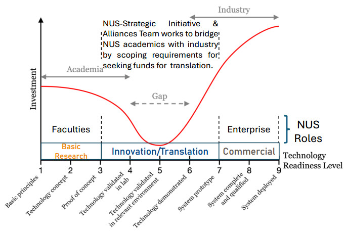
Campus as a Living Lab at the National University of Singapore is an initiative to bridge technologies from academia to industry across the valley of death [

| [1] | S. Nwaka, Technology readiness levels, the valley of death and scaling up innovations, In: Social and technological innovation in Africa, Singapore: Palgrave Macmillan, 2021, 99–107. https://doi.org/10.1007/978-981-16-0155-2_7 |
| [2] | The Business Times, Singapore spending Sfanxiexian_myfh25b in next five-year R and D plan, SPH Media, 2020. Available from: https://www.businesstimes.com.sg/singapore/economy-policy/singapore-spending-s25b-next-five-year-rd-plan. |
| [3] | National Research Foundation Singapore, Technology and Research, National Survey of Research, Innovation and Enterprise in Singapore 2021, Agency for Science, Technology and Research (A*STAR), 2024. Available from: https://www.a-star.edu.sg/docs/librariesprovider1/default-document-library/rie/2021-rie-survey-publication_finalforpublication_amended.pdf. |
| [4] | M. Teo, A. Loo, K. Leong, Economic Survey of Singapore: Third Quarter 2019, Ministry of Trade and Industry Republic of Singapore, 2019. Available from: https://www.mti.gov.sg/-/media/MTI/Resources/Economic-Survey-of-Singapore/2019/Economic-Survey-of-Singapore-Third-Quarter-2019/FullReport_3Q19.pdf. |
| [5] | P. Wong, Y. Ho, A. Singh, The impact of R & D on the Singaporean economy over 1978–2019, Singap. Econ. Rev., in press. https://doi.org/10.1142/S0217590823500480 |
| [6] | P. Wong, The development of Singapore's innovation and entrepreneurship ecosystem, In: Clusters of innovation in the age of disruption, Cheltenham: Edward Elgar Publishing, 2022,206–244. https://doi.org/10.4337/9781800885165.00019 |
| [7] | Ministry of Finance, Economy and Labour Market: Sustaining Singapore's global relevance and competitive edge, Government of Singapore, 2024. Available from: https://spor.performancereports.gov.sg/businesses/strong-and-resilient-economy/economy-and-labour-market. |
| [8] |
T. Tat, G. Ping, Innovating services and digital economy in Singapore, Commun. ACM, 63 (2020), 58–59. https://doi.org/10.1145/3378554 doi: 10.1145/3378554

|
| [9] | The University Campus Infrastructure (UCI) cluster of offices, Smart Safe Sustainable, National University of Singapore, 2019. Available from: https://uci.nus.edu.sg/wp-content/uploads/2024/03/Annual-report-2019-FINAL-BLUE.pdf. |
| [10] | M. Batty, Digital twins, Environ. Plan. B-Urban, 45 (2018), 817–820. https://doi.org/10.1177/2399808318796416 |
| [11] |
Y. Jiang, S. Yin, K. Li, H. Luo, O. Kaynak, Industrial applications of digital twins, Phil. Trans. R. Soc. A, 379 (2021), 20200360. https://doi.org/10.1098/rsta.2020.0360 doi: 10.1098/rsta.2020.0360
|
| [12] |
M. Juarez, V. Botti, A. Giret, Digital twins: review and challenges, J. Comput. Inf. Sci. Eng., 21 (2021), 030802. https://doi.org/10.1115/1.4050244 doi: 10.1115/1.4050244
|
| [13] | A Følstad, Living labs for innovation and development of information and communication technology: a literature review, Electronic Journal of Organizational Virtualness, 10 (2008), 99–131. |
| [14] |
M. Hossain, S. Leminen, M. Westerlund, A systematic review of living lab literature, J. Clean. Prod., 213 (2019), 976–988, https://doi.org/10.1016/j.jclepro.2018.12.257 doi: 10.1016/j.jclepro.2018.12.257
|
| [15] | P. Tay, N. Wang, TCI 2015 Innovation Clusters–-a National Strategy to Build Technology Capabilities in Singapore, SlideShare from Scribd, 2015. Available from: https://www.slideshare.net/slideshow/tci-2015-innovation-clusters-a-national-strategy-to-build-technology-capabilities-in-singapore/54947121. |
| [16] | R. Takken, One generic viewer for all current data types, GeoInformatics, 17 (2014), 44. |
| [17] | T. Ho, R. Yu, J. Lim, P. Fränti, Modelling implications & impacts of going green with EV in Singapore with multi-agent systems, Proceedings of Signal and Information Processing Association Annual Summit and Conference (APSIPA), 2014 Asia-Pacific, 2014, 1–6. https://doi.org/10.1109/APSIPA.2014.7041769 |
| [18] | W. Yang, T. Ho, L. Xiang, C. Chai, R. Yu, An overview and evaluation on demand response program in Singapore electricity market, Proceedings of IEEE Conference on Energy Conversion (CENCON), 2014, 61–66. https://doi.org/10.1109/CENCON.2014.6967477 |
| [19] |
H. Altalib, ROI calculations for electronic performance support systems, Perform. Improv., 41 (2002), 12–22. https://doi.org/10.1002/pfi.4140411005 doi: 10.1002/pfi.4140411005
|
| [20] |
B. Boehm, R. Valerdi, E. Honour, The ROI of systems engineering: some quantitative results for software‐intensive systems, Systems Eng., 11 (2008), 221–234. https://doi.org/10.1002/sys.20096 doi: 10.1002/sys.20096
|
| [21] |
G. Bockle, P. Clements, J. McGregor, D. Muthig, K. Schmid, Calculating ROI for software product lines, IEEE Software, 21 (2004), 23–31. https://doi.org/10.1109/MS.2004.1293069 doi: 10.1109/MS.2004.1293069
|
| [22] |
M. Tahmasebi, Cyberattack ramifications, the hidden cost of a security breach, Journal of Information Security, 15 (2024), 87–105. https://doi.org/10.4236/jis.2024.152007 doi: 10.4236/jis.2024.152007
|
| [23] | IBM and Ponemon Institute, Cost of a Data Breach: Report 2024, IBM, 2024. Available from: https://www.ibm.com/reports/data-breach. |


Figures(7)
Thomas Chee Tat Ho, George Chee Ping Loh. Translating research through the National University of Singapore campus as a living laboratory[J]. Applied Computing and Intelligence, 2025, 5(1): 82-93. doi: 10.3934/aci.2025006


 DownLoad: