Edge-assisted multi-user millimeter-wave radar for non-contact blood pressure monitoring

Xu Ji; Fang Dong; Zhaowu Huang; Xiaolin Guo; Haopeng Zhu; Baijun Chen; Jun Shen; Xu Ji; Fang Dong; Zhaowu Huang; Xiaolin Guo; Haopeng Zhu; Baijun Chen; Jun Shen

doi:10.3934/aci.2025004

Applied Computing and Intelligence

2025, Volume 5, Issue 1: 57-76. doi: 10.3934/aci.2025004

Previous Article Next Article

Research article

Edge-assisted multi-user millimeter-wave radar for non-contact blood pressure monitoring

1.
School of Computer Science and Engineering, Southeast University, Nanjing 211189, Jiangsu, China
2.
School of Computing and Information Technology, University of Wollongong, Wollongong, NSW, Australia

Academic Editor: Pasi Fränti

Received: 25 December 2024 Revised: 12 February 2025 Accepted: 13 February 2025 Published: 19 February 2025

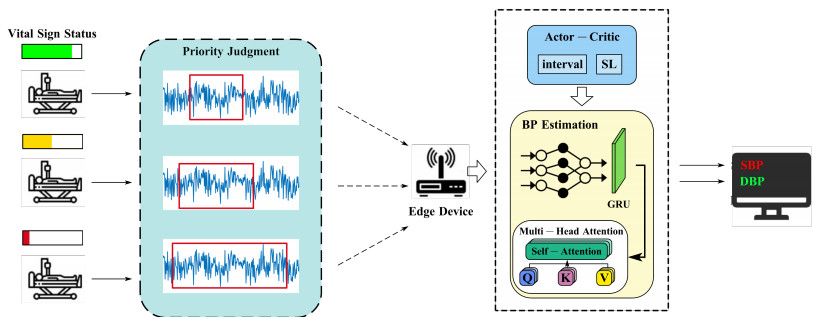
The non-contact blood pressure (BP) monitoring technology based on millimeter wave radar (mmWave) has been widely concerned for its advantages of non-invasive and real-time continuous monitoring. In recent years, studies have employed deep learning technologies to process mmWave radar, providing high-accuracy monitoring and high computing resource requirements. In this paper, we propose an edge-assisted framework for mmWave radar-based blood pressure monitoring to meet high accuracy and low latency application requirements because edge computing can provide a more powerful computing capability closer to users. However, it is non-trivial to effectively run such an edge-assisted mmWave radar-based blood pressure monitoring upon multiple users due to limited edge server resources. To solve this problem, we identify an opportunity to optimize the inference efficiency by adjusting key system parameters, such as sampling interval and input signal sequence length. This adjustment helps to reduce the inference latency and resource contention, especially in resource-constrained edge computing environments. By adaptively configuring these parameters for multiple users, we aim to strike a balance between a high accuracy and a low latency. First, we formulate the problem as an online learning problem and propose a deep reinforcement learning-based method to solve it. Finally, we implement a testbed to evaluate the performance of our method. Extensive experimental results show that our method outperforms the baselines, achieving a latency reduction of up to 70.3% and improving a reward by up to 29.7%, while maintaining an accuracy loss within 5%.
- millimeter-wave radar,
- blood pressure monitoring,
- edge computing,
- latency-sensitive,
- deep learning
Citation: Xu Ji, Fang Dong, Zhaowu Huang, Xiaolin Guo, Haopeng Zhu, Baijun Chen, Jun Shen. Edge-assisted multi-user millimeter-wave radar for non-contact blood pressure monitoring[J]. Applied Computing and Intelligence, 2025, 5(1): 57-76. doi: 10.3934/aci.2025004

Related Papers:

Abstract

The non-contact blood pressure (BP) monitoring technology based on millimeter wave radar (mmWave) has been widely concerned for its advantages of non-invasive and real-time continuous monitoring. In recent years, studies have employed deep learning technologies to process mmWave radar, providing high-accuracy monitoring and high computing resource requirements. In this paper, we propose an edge-assisted framework for mmWave radar-based blood pressure monitoring to meet high accuracy and low latency application requirements because edge computing can provide a more powerful computing capability closer to users. However, it is non-trivial to effectively run such an edge-assisted mmWave radar-based blood pressure monitoring upon multiple users due to limited edge server resources. To solve this problem, we identify an opportunity to optimize the inference efficiency by adjusting key system parameters, such as sampling interval and input signal sequence length. This adjustment helps to reduce the inference latency and resource contention, especially in resource-constrained edge computing environments. By adaptively configuring these parameters for multiple users, we aim to strike a balance between a high accuracy and a low latency. First, we formulate the problem as an online learning problem and propose a deep reinforcement learning-based method to solve it. Finally, we implement a testbed to evaluate the performance of our method. Extensive experimental results show that our method outperforms the baselines, achieving a latency reduction of up to 70.3% and improving a reward by up to 29.7%, while maintaining an accuracy loss within 5%.

References

[1]	D. S. Picone, Accurate measurement of blood pressure, Artery Res., 26 (2020), 130–136. https://doi.org/10.2991/artres.k.200624.001 doi: 10.2991/artres.k.200624.001
[2]	G. Mancia, G. Parati, Ambulatory blood pressure monitoring and organ damage, Hypertension, 36 (2000), 894–900. https://doi.org/10.1161/01.HYP.36.5.894 doi: 10.1161/01.HYP.36.5.894
[3]	N. Tomitani, S. Hoshide, K. Kario, The importance of regular home blood pressure monitoring over the life course, Hypertens. Res., 47 (2024), 540–542. https://doi.org/10.1038/s41440-023-01492-8 doi: 10.1038/s41440-023-01492-8
[4]	K. Kario, Morning surge in blood pressure and cardiovascular risk: evidence and perspectives, Hypertension, 56 (2010), 765–773. https://doi.org/10.1161/HYPERTENSIONAHA.110.157149 doi: 10.1161/HYPERTENSIONAHA.110.157149
[5]	S. Iyer, L. Zhao, M. P. Mohan, J. Jimeno, M. Y. Siyal, A. Alphones, et al., mm-wave radar-based vital signs monitoring and arrhythmia detection using machine learning, Sensors, 22 (2022), 3106. https://doi.org/10.3390/s22093106 doi: 10.3390/s22093106
[6]	M. Ebrahim, F. Heydari, T. Wu, K. Walker, K. Joe, J. Redoute, et al., Blood pressure estimation using on-body continuous wave radar and photoplethysmogram in various posture and exercise conditions, Sci. Rep., 9 (2019), 16346. https://doi.org/10.1038/s41598-019-52710-8 doi: 10.1038/s41598-019-52710-8
[7]	Y. Liang, A. Zhou, X. Wen, W. Huang, P. Shi, L. Pu, et al., Airbp: monitor your blood pressure with millimeter-wave in the air, ACM T. Internet Thing., 4 (2023), 28. https://doi.org/10.1145/3614439 doi: 10.1145/3614439
[8]	Y. Ran, D. Zhang, J. Chen, Y. Hu, Y. Chen, Contactless blood pressure monitoring with mmwave radar, Proceedings of IEEE Global Communications Conference (GLOBECOM), 2022,541–546. https://doi.org/10.1109/GLOBECOM48099.2022.10001592
[9]	U. Senturk, K. Polat, I. Yucedag, A non-invasive continuous cuffless blood pressure estimation using dynamic recurrent neural networks, Appl. Acoust., 170 (2020), 107534. https://doi.org/10.1016/j.apacoust.2020.107534 doi: 10.1016/j.apacoust.2020.107534
[10]	Q. Hu, Q. Zhang, H. Lu, S. Wu, Y. Zhou, Q. Huang, et al., Contactless arterial blood pressure waveform monitoring with mmwave radar, Proceedings of the ACM on Interactive, Mobile, Wearable and Ubiquitous Technologies, 8 (2024), 178. https://doi.org/10.1145/3699781 doi: 10.1145/3699781
[11]	A. Vaswani, N. Shazeer, N. Parmar, J. Uszkoreit, L. Jones, A. Gomez, et al., Attention is all you need, Proceedings of the 31st International Conference on Neural Information Processing Systems, 2017, 6000–6010.
[12]	A. Zhao, E. Zhu, R. Lu, M. Lin, Y. Liu, G. Huang, Augmenting unsupervised reinforcement learning with self-reference, arXiv: 2311.09692. https://doi.org/10.48550/arXiv.2311.09692
[13]	Z. Jiang, S. Li, L. Wang, F. Yu, Y. Zeng, H. Li, et al., A comparison of invasive arterial blood pressure measurement with oscillometric non-invasive blood pressure measurement in patients with sepsis, J. Anesth., 38 (2024), 222–231. https://doi.org/10.1007/s00540-023-03304-2 doi: 10.1007/s00540-023-03304-2
[14]	G. Van Montfrans, G. Van Der Hoeven, J. Karemaker, W. Wieling, A. Dunning, Accuracy of auscultatory blood pressure measurement with a long cuff, Br. Med. J. (Clin. Res. Ed.), 295 (1987), 354–355. https://doi.org/10.1136/bmj.295.6594.354 doi: 10.1136/bmj.295.6594.354
[15]	M. Ramsey, Noninvasive automatic determination of mean arterial pressure, Med. Biol. Eng. Comput., 17 (1979), 11–18. https://doi.org/10.1007/BF02440948 doi: 10.1007/BF02440948
[16]	J. Penaz, Photoelectric measurement of blood pressure, volume and flow in the finger, Proceedings of the 10th international conference on medical and biological engineering, 1973,104.
[17]	G. Pressman, P. Newgard, A transducer for the continuous external measurement of arterial blood pressure, IEEE Transactions on Biomedical Electronics, 10 (1963), 73–81. https://doi.org/10.1109/TBMEL.1963.4322794 doi: 10.1109/TBMEL.1963.4322794
[18]	I. Black, N. Kotrapu, H. Massie, Application of doppler ultrasound to blood pressure measurement in small infants, J. Pediatr., 81 (1972), 932–935. https://doi.org/10.1016/S0022-3476(72)80546-8 doi: 10.1016/S0022-3476(72)80546-8
[19]	Y. Cao, H. Chen, F. Li, Y. Wang, Crisp-bp: continuous wrist ppg-based blood pressure measurement, Proceedings of the 27th Annual International Conference on Mobile Computing and Networking, 2021,378–391. https://doi.org/10.1145/3447993.3483241 doi: 10.1145/3447993.3483241
[20]	N. Pilz, D. S. Picone, A. Patzak, O. S. Opatz, T. Lindner, L. Fesseler, et al., Cuff-based blood pressure measurement: challenges and solutions, Blood Pressure, 33 (2024), 2402368. https://doi.org/10.1080/08037051.2024.2402368 doi: 10.1080/08037051.2024.2402368
[21]	Z. Shi, T. Gu, Y. Zhang, X. Zhang, mmbp: contact-free millimetre-wave radar based approach to blood pressure measurement, Proceedings of the 20th ACM Conference on Embedded Networked Sensor Systems, 2023,667–681. https://doi.org/10.1145/3560905.3568506 doi: 10.1145/3560905.3568506
[22]	J. Zou, S. Zhou, B. Ge, X. Yang, Non-contact blood pressure measurement based on ippg, Journal of New Media, 3 (2021), 41–51. https://doi.org/10.32604/jnm.2021.017764 doi: 10.32604/jnm.2021.017764
[23]	L. Xu, P. Wu, P. Xia, F. Geng, P. Wang, X. Chen, et al., Continuous and noninvasive measurement of arterial pulse pressure and pressure waveform using an image-free ultrasound system, arXiv: 2305.17896. https://doi.org/10.48550/arXiv.2305.17896
[24]	M. Alizadeh, G. Shaker, J. De Almeida, P. Morita, S. Safavi-Naeini, Remote monitoring of human vital signs using mm-wave fmcw radar, IEEE Access, 7 (2019), 54958–54968. https://doi.org/10.1109/ACCESS.2019.2912956 doi: 10.1109/ACCESS.2019.2912956
[25]	S. Churkin, L. Anishchenko, Millimeter-wave radar for vital signs monitoring, Proceedings of IEEE International Conference on Microwaves, Communications, Antennas and Electronic Systems (COMCAS), 2015, 1–4. https://doi.org/10.1109/COMCAS.2015.7360366 doi: 10.1109/COMCAS.2015.7360366
[26]	Z. Ling, W. Zhou, Y. Ren, J. Wang, L. Guo, Non-contact heart rate monitoring based on millimeter wave radar, IEEE Access, 10 (2022), 74033–74044. https://doi.org/10.1109/ACCESS.2022.3190355 doi: 10.1109/ACCESS.2022.3190355
[27]	F. Shamsfakhr, D. Macii, L. Palopoli, M. Corrà, A. Ferrari, D. Fontanelli, A multi-target detection and position tracking algorithm based on mmwave-fmcw radar data, Measurement, 234 (2024), 114797. https://doi.org/10.1016/j.measurement.2024.114797 doi: 10.1016/j.measurement.2024.114797

Reader Comments

Your name:*

Email:*
© 2025 the Author(s), licensee AIMS Press. This is an open access article distributed under the terms of the Creative Commons Attribution License (http://creativecommons.org/licenses/by/4.0)