
Citation: Fiammetta Iannuzzo, Silvia Crudo, Gianpaolo Antonio Basile, Fortunato Battaglia, Carmenrita Infortuna, Maria Rosaria Anna Muscatello, Antonio Bruno. Efficacy and safety of non-invasive brain stimulation techniques for the treatment of nicotine addiction: A systematic review of randomized controlled trials[J]. AIMS Neuroscience, 2024, 11(3): 212-225. doi: 10.3934/Neuroscience.2024014
[1] | Evgenii Lukin, Ekaterina Leonidova, Elena Shirokova, Nikita Rumyantsev, Maksim Sidorov . Russian economy under sanctions (Case of the northwest of Russia). National Accounting Review, 2023, 5(2): 145-158. doi: 10.3934/NAR.2023009 |
[2] | Guido Ferrari, Yanyun Zhao, José Mondéjar Jiménez, Luca Secondi . The economy of Tuscany in the post Covid-19 era: struggling with energy crisis and inflation. What to do to resume the journey?1. National Accounting Review, 2024, 6(1): 1-26. doi: 10.3934/NAR.2024001 |
[3] | Sylvie Kotíková, Roman Vavrek . Development of foreign direct investment in the context of government aid: A case study of the Czech Republic since 1998. National Accounting Review, 2025, 7(2): 196-220. doi: 10.3934/NAR.2025009 |
[4] | Sylvie Kotíková . Spillover effects: A challenging public interest to measure. National Accounting Review, 2023, 5(4): 373-404. doi: 10.3934/NAR.2023022 |
[5] | Ming He, Barnabé Walheer . Technology intensity and ownership in the Chinese manufacturing industry: A labor productivity decomposition approach. National Accounting Review, 2020, 2(2): 110-137. doi: 10.3934/NAR.2020007 |
[6] | Yanyun Zhao, Bingjie Liu . The evolution and new trends of China's tourism industry. National Accounting Review, 2020, 2(4): 337-353. doi: 10.3934/NAR.2020020 |
[7] | Dina Krasnoselskaya, Venera Timiryanova . Exploring the impact of ecological dimension on municipal investment: empirical evidence from Russia. National Accounting Review, 2023, 5(3): 227-244. doi: 10.3934/NAR.2023014 |
[8] | Mengxin Wang, Lang Li, Hanyong Lan . The measurement and analysis of technological innovation diffusion in China's manufacturing industry. National Accounting Review, 2021, 3(4): 452-471. doi: 10.3934/NAR.2021024 |
[9] | Jiehua Ma, Zhenghui Li . Measuring China's urban digital economy. National Accounting Review, 2022, 4(4): 329-361. doi: 10.3934/NAR.2022019 |
[10] | Yanting Xu, Tinghui Li . Measuring digital economy in China. National Accounting Review, 2022, 4(3): 251-272. doi: 10.3934/NAR.2022015 |
Ever since the studies of epidemiology conducted by Kermack et al. [1] mathematical models have become important tools for studying the spread and control of infectious diseases. For some deterministic epidemic models, many researchers have studied the dynamical behaviors [1,2,3,4,5,6]. Moreover, Chen et al. [9] proposed that the coefficient of deterministic epidemic system may be influenced by stochastic perturbation. Therefore, stochastic models have been studied to find out impacts of stochastic fluctuation upon the infectious diseases [11,11,24,29,30]. For example, the studies conducted by Zhao et al. [11] on the asymptotic behavior of a stochastic SIS epidemic model with vaccination. Cai et al. [11] proves the existence of stationary distribution of a stochastic SIRS epidemic model.
In fact, some parameters of the epidemic models may be influenced by the sudden changes such as color noise which deems to be a random switching from one environment regime to another under the influence of such factors as temperature or rainfall [15,17]. For the first equation of the SIV epidemic model, the parameters are determined as follows:
dS(t)=((1−p)μ+αI(t)−(μ+u1)S(t)−βS(t)I(t))dt−σS(t)I(t)dB(t), | (1.1) |
we assume that there are n regimes and the system obeys
dS(t)=((1−p(1))μ(1)+α(1)I(t)−(μ(1)+u1(1))S(t)−β(1)S(t)I(t))dt−σ(1)S(t)I(t)dB(t), | (1.2) |
when it is in regime 1, while it obeys another stochastic model
dS(t)=((1−p(2))μ(2)+α(2)I(t)−(μ(2)+u1(2))S(t)−β(2)S(t)I(t))dt−σ(2)S(t)I(t)dB(t), | (1.3) |
in regime 2 and so on. Therefore, the system obeys
dS(t)=((1−p(i))μ(i)+α(i)I(t)−(μ(i)+u1(i))S(t)−β(i)S(t)I(t))dt−σ(i)S(t)I(t)dB(t) | (1.4) |
in regime i(1≤i≤n). To best reveal the way the environment noise affects the epidemic systems, we propose the application of continuous-time Markov chain to define this phenomenon [18,19,20]. It is significant to study the effect of random switching of environmental regimes on the spread dynamic of diseases.
As it is known that SIV epidemic model has drawn much attention. For instance, Liu et al. [26] discussed the existence and uniqueness of the global positive solution of the system, and Lin et al. [23] considered the asymptotic stability of the stochastic SIV epidemic model and the existence of a stationary distribution. The above work done just focused on the studies of dynamic behaviors of SIV system with quite few studies focusing on the optimal control for stochastic SIV models with Markov chains. The study of optimal control of stochastic SIV epidemic model, therefore, becomes significant.
In addition, vaccination and treatment have become the most effective strategies in the control of the epidemic transmission. We give priority to vaccinations to susceptible people. Vaccination duration and effective treatment make it possible to curb the spread of diseases and cut the cost of vaccines. For instance, Measles is a highly contagious disease that may result in serious illness in the early childhood stage, and therefore the advance immunization is necessary [25]. The global Measles and Rubella Strategic Plan 2012–2020, aims to reduce global measles mortality and to achieve measles elimination by the end of the 2020 (http://www.measlesinitiative.org/). The most effective approach to achieve this plan is vaccination. In view of this above, it is meaningful to carry out the research of a stochastic SIV epidemic model with vaccination and saturated treatment to analyze the near-optimal control with Markov chains.
According to the paper, the objective function is determined and constructed on the basis of an optimal control problem with two control variables of vaccination and treatment. And the optimal solution of the model is provided according to the objective function through analysis in the relevant optimal theories. Aiming at the stochastic SIV model with Markov chain, we carried out thorough studies on the minimization of the number of infected individuals through the application of prophylactic vaccination and saturated treatment. We also define the sufficient and necessary conditions for the near-optimal control problems. The innovative ideas of the study are as follows:
● Provision of an innovative stochastic SIV epidemic model with vaccination, treatment and Markov chains;
● Discussion of sufficient and necessary conditions of the near-optimal control for a stochastic SIV model.
The remaining part of of the paper is so organized as: Section 2 preliminaries and introduction of stochastic SIV model; Section 3 proof of the necessary condition for near-optimal control; Section 4, institution of sufficient conditions for near-optimal control; Section 5 numerical simulations display to confirm the results; and, Section 6, conclusions.
In this section, we first introduce the following notations and definitions before we formulate the model.
We define (Ω,F,F0≤t≤T,P) be a complete filtered probability space on a finite time horizon [0,T]. We assume (Ft)0≤t≤T is the natural filtration and F=FT, Uad is the set of all admissible controls, fx denotes the partial derivative of f with respect to x, |⋅| denotes the norm of an Euclidean space, XS denotes the indicator function of a set S, X+Y is the set {x+y: x∈X, y∈Y} for any sets X and Y, C is the different parameters in the paper.
We establish the optimal problems on the basis of a stochastic SIV model was put forward by Safan and Rihan et al. [14] as follows:
{dS(t)=[(1−p)μ+αI(t)−(μ+u1)S(t)−βS(t)I(t)]dt,dI(t)=[βS(t)I(t)+(1−e)βV(t)I(t)−(μ+α)I(t)]dt,dV(t)=[pμ+u1S(t)−μV(t)−(1−e)βV(t)I(t)]dt. | (2.1) |
with initial conditions S(0)≥0,I(0)≥0, and V(0)≥0. The population size is denoted by N(t) with N(t)=S(t)+I(t)+V(t). The SIV model assume that recovered individuals may lose immunity and move into the susceptible class again. Note that 0≤p≤1 and βS(t)I(t) is the incidence rate. Vaccinated individuals can either die with rate μ or obtain infected with force of infection (1−e)βI where e measures the efficacy of the vaccine induced protection against infection. If e=1, then the vaccine is perfectly effective in preventing infection, while e=0 means that the vaccine has no effect. The following flux diagram (Figure 1) illustrating the transmission of susceptible, infected and vaccinated. S, I and V represent susceptible, infected and vaccinated respectively. The continuous line represents nonlinear transmission rate between different compartments.
We assume that stochastic perturbations in the environment will mainly affect the parameter β, as in Tornatore et al. [27], so that β→β+σ˙B(t), where B(t) is a standard Brownian motion with the intensity σ2>0. All parameters in model (2.1) are assumed to be positive due to the physical meaning and more precisely are listed in Table.1. By this way, the stochastic version corresponding to system (2.1) be expressed by Liu et al. [26] as follows:
{dS(t)=[(1−p)μ+αI(t)−(μ+u1)S(t)−βS(t)I(t)]dt−σS(t)I(t)dB(t),dI(t)=[βS(t)I(t)+(1−e)βV(t)I(t)−(μ+α)I(t)]dt+σS(t)I(t)dB(t)+(1−e)σV(t)I(t)dB(t),dV(t)=[pμ+u1S(t)−μV(t)−(1−e)βV(t)I(t)]dt−(1−e)σV(t)I(t)dB(t). | (2.2) |
Parameters | Biological meanings |
p | The proportion of population that get vaccinated immediately after birth |
u1 | Vaccinated rate |
β | Per capita transmission coefficient |
μ | Per capita natural death rate / birth rate |
α | Per capita recovery rate |
σ | The intensities of the white noise |
S(t) | Susceptible proportion in the total population |
I(t) | Infected proportion in the total population |
V(t) | Vaccinated proportion in the total population |
According to [28], we know that the switching of the Markov chain is memoryless and the waiting time for the next switch is subjected to an exponential distribution. In addition, we assume that there are N regimes and the switching between them is governed by a Markov chain on the state space S={1,2,...,N}. Then as the sample path of Markov chain ξ(t) is right continuous step function almost surely, its jump points have no accumulation point. Thus, there exists a stopping sequence {τk}k≥0 for every w∈Ω, and a finite random constant ˉk=ˉk(w) such that 0=τ0<τ1...<τˉk=τ. Then when k>ˉk, we get that τk>τ and ξ(t) is a random constant in every intervals. That is to say, ξ(t)=ξ(τk) for τk≤t≤τk+1.
Let Rn+={x∈Rn:xi>0,i=1,2,...,n}, and |x|=√∑ni=1x2i. Then Markov process (x(t),ξ(t))∈Rn+×S, making up a diffusion component x(t) and a jump component ξ(t), can be described as follows:
{dx(t)=f(x(t),ξ(t))dt+g(x(t),ξ(t))dB(t),x(0)=x0∈Rn+,ξ(0)=ˉw∈S, | (2.3) |
where B(t) is a d-dimensional Brownian motion, and f(⋅,⋅):Rn×S⟶Rn, g(⋅,⋅):Rn×S⟶Rn×d.
If for any twice continuously differentiable function V(x,k)∈C2(Rn×S), define linear operator L by
LV(x,k)=n∑j=1fj(x,i)∂V(x,i)∂xj+12n∑j,k=1ajk(x,i)∂2V(x,i)∂xixj+∑j≠k∈Sqkj(x)(V(x,j)−V(x,k)), |
where a(x,i)=g(x,i)g⊤(x,i) with the superscript T stands for the transpose of a matrix or vector.
Hypothesis. The following basic hypothesis need to be satisfied
(H1) For all 0≤t≤T, the partial derivatives Lx1(t)(t,x(t);u(t)), Lx2(t)(t,x(t);u(t)), and Lx3(t)(t,x(t);u(t)) are continuous, and there is a constant C such that
|A1+A2|≤C(1+|x1(t)+x2(t)+x3(t)|). |
(H2) Let x(t), x′(t)∈R3+ and ui(t), u′i(t)∈Uad,i=1,2, then for any 0≤t≤T, the function L(t,x(t);u(t)) is differentiable in u(t), and there exists a constant C such that
|hx2(t)(x(t))−hx′2(t)(x′(t))|≤C|x2(t)−x′2(t)|. |
(H3) The control set Uad is convex.
(H4) Assume that
Π=∑l∈Mπk(μ(k)+12σ21(k)+(μ(k)+α(k))+12σ22(k)+(μ(k)+α(k))+12σ23(k))>0, | (2.4) |
holds.
(H5) Assume that
K=(1−p(k))b(k)x1(t)−β(k)x2(t)1+x22(t)+α(k)x3(t)x1(t)−u1(t)−12σ24(k)x22(t)(1+x22(t))2+β(k)x1(t)1+x22(t)−12σ24(k)x21(t)(1+x22(t))2+p(k)b(k)x3(t)−m(k)u2(t)1+η(k)x2(t)+u1(t)x1(t)x3(t)+m(k)u2(t)x2(t)(1+η(k)x2(t))x3(t)+α(k)x2(t)x3(t)<0, | (2.5) |
holds. We introduce the treatment control u2(t) into the above model (2.2). With the help of vaccination or treatment, the number of susceptible individuals increased, using Su represent it. In fact, every community should have proper treatment ability. If investment in treatment is too large, the community will pay unnecessary expenses. If it is too small, the community will have the risk of disease outbreaks. Therefore, it is very important to determine the right treatment ability. Following Wang's argument in [22], the advantage of using a saturated type treatment function is that it generates near-linear treatment results. We assume that the treatment function is a function of u2(t) and I(t). It is defined as T(u2(t),I(t))=mu2(t)I(t)1+ηI(t), where m>0,η≥0. Our new model is as follows:
{dS(t)=((1−p)μ+αI(t)−(μ+u1(t))S(t)−βS(t)I(t))dt−σS(t)I(t)dB1(t)dI(t)=(βS(t)I(t)+(1−e)βV(t)I(t)−(μ+α)I(t)−mu2(t)I(t)1+ηI(t))dt−σS(t)I(t)dB2(t)+(1−e)σV(t)I(t)dB4(t),dV(t)=(pμ−μV(t)−(1−e)βV(t)I(t)+u1(t)S(t)+mu2(t)I(t)1+ηI(t))dt−(1−e)σV(t)I(t)dB3(t). | (2.6) |
where m is the cure rate, η in the treatment function measures the extent of delayed treatment given to infected people. Let U⊆R be a bounded nonempty closed set. The control u(t)∈U is called admissible, if it is an Ft-adapted process with values in U. The set of all admissible controls is denoted by Uad. In this optimal problem, we assume a restriction on the control variable such that 0≤u1(t)≤0.9 [12], because it is impossible for all susceptible individuals to be vaccinated at one time. u2(t)=0 represents no treatment, and u2(t)=1 represents totally effective treatment.
For the sake of showing such sudden environmental abrupt shift in different regimes, we will introduce the colored noise (i.e. the Markov chain) into the SIV epidemic model (2.6). Let ξ(t) be a right-continuous Markov chain in a finite state space S={1,2,...,N} with generator α=(qij)N×N given by
P{ξ(t+Δt)=j|ξ(t)=i}={qijΔt+o(Δ), if j≠i,1+qiiΔt+o(Δ), if j=i, | (2.7) |
where Δt>0 and qij is the transition rate from state i to state j and qij≥0 if j≠i while qii=−∑j≠iqij.
Then we can obtain the novel SIV epidemic model as follows:
{dS(t)=((1−p(ξ(t)))μ(ξ(t))+α(ξ(t))I(t)−(μ(ξ(t))+u1(t))S(t)−β(ξ(t))S(t)I(t))dt−σ(ξ(t))S(t)I(t)dB1(t),dI(t)=(β(ξ(t))S(t)I(t)+(1−e)β(ξ(t))V(t)I(t)−(μ(ξ(t))+α(ξ(t)))I(t)−m(ξ(t))u2(t)I(t)1+η(ξ(t))I(t))dt−σ(ξ(t))S(t)I(t)dB2(t)+(1−e)σ(ξ(t))V(t)I(t)dB4(t),dV(t)=(p(ξ(t))μ(ξ(t))+u1(t)S(t)−μ(ξ(t))V(t)−(1−e)β(ξ(t))V(t)I(t)+m(ξ(t))u2(t)I(t)1+η(ξ(t))I(t))dt−(1−e)σ(ξ(t))V(t)I(t)dB3(t). | (2.8) |
To simplify equations, we represent xi(t)=(x1(t),x2(t),x3(t))⊤=(S(t),I(t),V(t))⊤, u(t)=(u1(t),u2(t))⊤ and the model (2.8) can be rewritten as
{dx1(t)=((1−p(ξ(t)))μ(ξ(t))+α(ξ(t))x2(t)−μ(ξ(t))x1(t)−β(ξ(t))x1(t)x2(t)−u1(t)x1(t))dt−σ(ξ(t))x1(t)x2(t)dB1(t)≡f1(x(t),u(t))dt−σ14(x(t))dB(t),dx2(t)=(β(ξ(t))x1(t)x2(t)+(1−e)β(ξ(t))x2(t)x3(t)−(μ(ξ(t))+α(ξ(t)))x2(t)−m(ξ(t))u2(t)x2(t)1+η(ξ(t))x2(t))dt−σ(ξ(t))x1(t)x2(t)dB2(t)+(1−e)σ(ξ(t))x2(t)x3(t)dB4(t)≡f2(x(t),u(t))dt−σ24(x(t))dB(t),dx3(t)=(p(ξ(t))μ(ξ(t))+u1(t)x1(t)−μ(ξ(t))x3(t)−(1−e)β(ξ(t))x2(t)x3(t)+m(ξ(t))u2(t)x2(t)1+η(ξ(t))x2(t))dt−(1−e)σ(ξ(t))x2(t)x3(t)dB3(t)≡f3(x(t),u(t))dt−σ34(x(t))dB(t),x(0)=x0. | (2.9) |
with the objective function
J(0,x0;u(t))=E(∫T0L(x(t),u(t))dt+h(x(T))), | (2.10) |
where x(t)={x(t):0≤t≤T} is the solution of model (2.9) on the filtered space (Ω,F,(Ft)0≤t≤T,P). For any u(t)∈Uad, model (2.9) has a unique Ft-adapted solution x(t) and (x(t),u(t)) is called an admissible pair. The control problem is to find an admissible control which minimizes or nearly minimizes the objective function J(0,x0;u(⋅)) over all u(⋅)∈Uad. The objective function J(0,x0;u(⋅)) represent a function that t=0,x(t)=x0 with control variable u(⋅). The value function is as follows:
V(0,x0)=minu(⋅)∈UadJ(0,x0;u(⋅)). |
Our goal is to minimize the total number of the infected and susceptible individuals by using minimal control efforts. Refering to Lashari et al. [13], let the objective function in this paper is
J(0,x0;u(t))=E{∫T0(A1S(t)+A2I(t)+12(τ1u21(t)+τ2u22(t)))dt+h(x(T))}, | (2.11) |
where τ1 and τ2 are positive constants,
L(x(t),u(t))=A1S(t)+A2I(t)+12(τ1u21(t)+τ2u22(t)),h(x(T))=(0,I(T),0). |
Definition 2.1. (Optimal Control) [7]. If u∗(⋅) or an admissible pair(x∗(t),u∗(t)) attains the minimum of J(0,x0;u(⋅)), then an admissible control u∗(⋅) is called optimal.
Definition 2.2. (ε-Optimal Control) [7]. For a given ε>0, an admissible pair(x∗(t),u∗(t)) or an admissible control uε(⋅) is called ε-optimal, if
|J(0,x0;uε(⋅))−V(0,x0)|≤ε. |
Definition 2.3. (Near-optimal Control) [7]. A family of admissible controls {uε(⋅)} parameterized by ε>0 and any element (x∗(t),u∗(t)), or any element uε(⋅) in the family are called near-optimal, if
|J(0,x0;uε(⋅))−V(0,x0)|≤δ(ε), |
holds for a sufficiently small ε>0, where δ is a function of ε satisfying δ(ε)→0 as ε→0. The estimate δ(ε) is called an error bound. If δ(ε)=cεκ for some c,κ>0, then uε(⋅) is called near-optimal with order εκ.
Definition 2.4. [11]. Let Ξ⊂Rn be a region and u1:Ξ⟶Rn be a locally Lipschitz continuous function. The generalized gradient of ϕ at ξ∈Ξ is defined as
∂ϕ(ξ)={ζ∈Rn|⟨ζ,η⟩≤¯limy→ξ,y∈Ξ,m↓0ϕ(y+mη)−ϕ(y)m}. |
Our next goal is to derive a set of necessary conditions for near-optimal controls.
In this section, we will introduce two lemmas at first, then we will obtain the necessary condition for the near-optimal control of the model (2.8).
Lemma 3.1. For all θ≥0 and 0<κ<1 satisfying κθ<1, and u(t),u′(t)</italic><italic>∈Uad, along with the corresponding trajectories x(t),x′(t), there exists a constant C=C(θ,κ) such that
3∑i=1Esup0≤t≤T|xi(t)−x′i(t)|2θ≤C2∑i=1d(ui(t),u′i(t))κθ. | (3.1) |
Proof. We assume θ≥1 and ∀r>0, use the elementary inequality, and get
Esup0≤t≤r |x1(t)−x′1(t)|2θ≤CE∫r0[(β2θ(ξ(t))+σ2θ4(ξ(t)))|x1(t)x2(t)1+x22(t)−x′1(t)x′2(t)1+x′22(t)|2θ+(μ2θ1(ξ(t))−σ2θ2(ξ(t)))|x1(t)−x′1(t)|2θ+α2θ(ξ(t))|x3(t)−x′3(t)|2θ+|u1(t)x1(t)−u′1(t)x′1(t)|2θ]dt≤CE∫r03∑i=1|xi(t)−x′i(t)|2θdt+C[E∫r0χu1(t)≠u′1(t)(t)dt]κθ≤C[E∫r03∑i=1|xi(t)−x′i(t)|2θdt+d(u1(t),u′1(t))κθ]. | (3.2) |
If 0<κ<1, then θ≥1, we apply Cauchy-Schwartz's inequality and get
E∫r0χu1(t)≠u′1(t)(t)dt≤C(E∫r0dt)1−κθ×(E∫r0χu1(t)≠u′1(t)(t)dt)κθ≤Cd(u1(t),u′1(t))κθ. | (3.3) |
Similarly, we can get the following estimates for |xi(t)−x′i(t)|2θ(i=2,3)
Esup0≤t≤r |x2(t)−x′2(t)|2θ≤C[E∫r02∑i=1|xi(t)−x′i(t)|2θdt+d(u2(t),u′2(t))κθ],Esup0≤t≤r |x3(t)−x′3(t)|2θ≤C[E∫r03∑i=2|xi(t)−x′i(t)|2θdt+2∑i=1d(ui(t),u′i(t))κθ]. | (3.4) |
Then, summing up (3.2) and (3.4), we may obtain that
3∑i=1Esup0≤t≤r |xi(t)−x′i(t)|2θ≤C[∫r03∑i=1Esup0≤t≤s|xi(t)−x′i(t)|2θds+2∑i=1d(ui(t),u′i(t))κθ]. |
Now by considering 0≤θ<1, with the help of Cauchy-Schwartz's inequality, we have
3∑i=1Esup0≤t≤r |xi(t)−x′i(t)|2θ≤3∑i=1[Esup0≤t≤r |xi(t)−x′i(t)|2]θ≤C[∫r03∑i=1Esup0≤t≤s|xi(t)−x′i(t)|2θds+2∑i=1d(ui(t),u′i(t))κ]θ≤Cθ[2∑i=1d(ui(t),u′i(t))κθ]. | (3.5) |
Therefore, the result is true by making use of Gronwall's inequality.
The proof is completed.
Lemma 3.2. Let Hypotheses (H3) and (H4) hold. For all 0<κ<1 and 0<θ<2 satisfying (1+κ)θ<2, and u(t),u′(t)∈Uad, along with the corresponding trajectories x(t),x′(t), and the solution (p(t),q(t)),(p′(t),q′(t)) of corresponding adjoint equation, there exists a constant C=C(κ,θ)>0 such that
3∑i=1E∫T0|pi(t)−p′i(t)|θdt+3∑i=1E∫T0|qi(t)−q′i(t)|θdt≤C2∑i=1d(ui(t),u′i(t))κθ2. | (3.6) |
Proof. Let ˆpi(t)≡pi(t)−p′i(t),ˆqj(t)≡qj(t)−q′j(t)(i,j=1,2,3). From the adjoint equation (4.5), we have
{dˆp1(t)=−[−((μ(ξ(t))+u1(t))x1(t)+β(ξ(t))x2(t)+μ(ξ(t)))ˆp1(t)+β(ξ(t))x2(t)ˆp2(t)+u1(t)ˆp3(t)−σ(ξ(t))x2(t)ˆq1(t)+σ(ξ(t))x2(t)ˆq2(t)+ˆf1(t)]dt+ˆq1(t)dB(t),dˆp2(t)=−[(α(ξ(t))−β(ξ(t))x1(t))ˆp1(t)+(β(ξ(t))x1(t)−(1−e)β(ξ(t))x3(t)−(μ(ξ(t))+α(ξ(t)))−m(ξ(t))u2(t)x2(t)1+η(ξ(t))x2(t))ˆp2(t)−((1−e)β(ξ(t))x3(t)−m(ξ(t))u2(t)x2(t)1+η(ξ(t))x2(t))ˆp3(t)−σ(ξ(t))x1(t)ˆq1(t)+(σ(ξ(t))x1(t)+(1−e)σ(ξ(t))x3(t))ˆq2(t)−((1−e)σ(ξ(t))x3(t))ˆq3(t)+ˆf2(t)]dt+ˆq2(t)dB(t),dˆp3(t)=−[((1−e)β(ξ(t))x2(t))ˆp2(t)−(μ(ξ(t))+(1−e)β(ξ(t))x2(t)ˆp3(t)]dt+((1−e)σ(ξ(t))x2(t))ˆq2(t)+((1−e)σ(ξ(t))x2(t))ˆq3(t)+ˆf3(t)+ˆq3(t)dB(t). | (3.7) |
where
ˆf1(t)=β(ξ(t))(x2(t)−x′2(t))(p′2(t)−p′1(t))+σ(ξ(t))(x2(t)−x′2(t))(q′2(t)−q′1(t)),ˆf2(t)=β(ξ(t))(x1(t)−x′1(t))(p′2(t)−p′1(t))+(1−e)β(ξ(t))(x3(t)−x′3(t))(p′3(t)−p′2(t))+m(ξ(t))x(u2(t)(1+η(ξ(t))x2(t))2−u′2(t)(1+η(ξ(t))x′2(t))2)(p′3(t)−p′2(t))+σ(ξ(t))(x1(t)−x′1(t))(q′2(t)−q′1(t))+(1−e)σ(ξ(t))(x3(t)−x′3(t))(q′3(t)−q′2(t)),ˆf3(t)=(1−e)β(ξ(t))(x2(t)−x′2(t))(p′2(t)−p′3(t))+(1−e)σ(ξ(t))(x2(t)−x′2(t))(q′2(t)−q′3(t)), |
We assume the solution of the following stochastic differential equation is ϕ(t)=(ϕ1(t),ϕ2(t),ϕ3(t))⊤.
{dϕ1(t)=−[((μ(ξ(t))+u1(t))x1(t)+β(ξ(t))x2(t)+μ(ξ(t)))ϕ1(t)+(α(ξ(t))−β(ξ(t))x1(t))ϕ2(t)+|ˆp1(t)|θ−1sgn(ˆp1(t))]dt+[(−σ(ξ(t))x2(t))ϕ1(t)+(−σ(ξ(t))x1(t))ϕ2(t)+|ˆq1(t)|θ−1sgn(ˆq1(t))]dB(t),dϕ2(t)=[β(ξ(t))x2(t)ϕ1(t)+(β(ξ(t))x1(t)−(1−e)β(ξ(t))x3(t)−(μ(ξ(t))+α(ξ(t)))−m(ξ(t))u2(t)x2(t)1+η(ξ(t))x2(t))ϕ2(t)+(1−e)β(ξ(t))x2(t)ϕ3(t)+|ˆp2(t)|θ(ξ(t))−1sgn(ˆp2(t))]dt+[σ(ξ(t))x2(t)ϕ1+(σ(ξ(t))x1(t)+(1−e)σ(ξ(t))x3(t))ϕ2+(1−e)σ(ξ(t))x2(t)ϕ3+|^q2|θ−1sgn(ˆq2(t)]dB(t),dϕ3(t)=[u1(t)ϕ1−((1−e)β(ξ(t))x3(t)−m(ξ(t))u2(t)x2(t)1+η(ξ(t))x2(t))ϕ2−(μ(ξ(t))+(1−e)β(ξ(t))x2(t))ϕ3+|ˆp3(t)|θ−1sgn(ˆp3(t))]dt+((−(1−e)σ(ξ(t))x3(t))ϕ1+(−(1−e)σ(ξ(t))x2(t))ϕ2+|ˆq3(t)|θ−1sgn(ˆq3(t)))dB(t), | (3.8) |
where sgn(⋅) is a symbolic function.
According to Hypothesis (H1), the definition of L and Lemma 4.2, the above equation admits a unique solution. Meanwhile, Cauchy-Schwartz's inequality indicates that
3∑i=1Esup0≤t≤T|ϕi(t)|θ1≤3∑i=1E∫T0 |ˆpi(t)|θdt+3∑i=1E∫T0 |ˆqi(t)|θdt, | (3.9) |
where θ1>2 and 1θ1+1θ=1.
In order to obtain the above inequality (3.6), we define the function
V(x(t),ˆp(t),ϕ(t),ˆq(t),k)=3∑i=1ˆpi(t)ϕi(t)+3∑i=1lnxi(t)+(¯wk+|ˉw|)=V1(x(t),ˆp(t),ϕ(t),ˆq(t))+V2(x(t))+V3(k), | (3.10) |
where ˉw=(ˉw1,ˉw2,⋯,ˉwN)⊤, |ˉw|=√ˉw21+⋯+ˉw2N and ¯wk(k∈S) are to be determined later and the reason for |ˉw| being is to make ¯wk+|ˉw| non-negative. Using Itô's formula [4] yields
LV1(x(t),ˆp(t),ϕ(t),ˆq(t))=3∑i=1E |ˆpi(t)|θ+2∑i=1E |ˆqi(t)|θ−3∑i=1E ˆfi(t)ϕi(t), | (3.11) |
LV2(x(t))=(1−p(k))μ(k)x1(t)+αx2(t)x1(t)−μ(k)−β(k)x2(t)−u1(t)+β(k)x1(t)+(1−e)β(k)x3(t)−(μ(k)+α(k))−m(k)u2(k)1+η(k)x2(t)+p(k)μ(k)x3(t)+u1(k)x1(t)x3(t)−μ(k)−(1−e)β(k)x2(t)+m(k)u2(k)x2(t)(1+η(k)x2(t))x3(t)−12σ2(k)x22(t)+12σ2(k)x21(t)+12(1−e)2σ(k)x23(t)−12(1−e)2σ2(k)x22(t)=K−(μ(k)+12σ21(k)+(μ(k)+α(k))+12σ22(k)+(μ(k)+α(k))+12σ23(k)), | (3.12) |
LV3(k)=∑l∈Mαkl¯wl. | (3.13) |
We define a vector Ξ=(Ξ1,Ξ2,⋯,ΞN)⊤ with
Ξk=μ(k)+12σ21(k)+(μ(k)+α(k))+12σ22(k)+(μ(k)+α(k))+12σ23(k). | (3.14) |
Due to the generator matrix α is irreducible and Lemma 2.3 in [5], for Ξk there exists a solution
ˉw=(¯w1,¯w2,⋯,¯wN)⊤, |
for the following poisson systems:
αˉw−Ξk=−∑Nj=1πjΞj. |
Thus, we obtain that
∑l∈Mαkl¯wl−(μ(k)+12σ21(k)+(μ(k)+α(k))+12σ22(k)+(μ(k)+α(k))+12σ23(k))=−∑l∈Mπk(μ(k)+12σ21(k)+(μ(k)+α(k))+12σ22(k)+(μ(k)+α(k))+12σ23(k))=−Π. | (3.15) |
According to Hypotheses (H4) and (H5), we get that
LV(x(t),p(t),q(t),k)=LV1(x(t),ˆp(t),ϕ(t),ˆq(t))+LV2(x(t))+LV3(k)=−Π+3∑i=1E |ˆpi(t)|θ+2∑i=1E |ˆqi(t)|θ−3∑i=1E ˆfi(t)ϕi(t)+K≤3∑i=1E |ˆpi(t)|θ+2∑i=1E |ˆqi(t)|θ−3∑i=1E ˆfi(t)ϕi(t). | (3.16) |
Integrating both side of (3.16) from 0 to T and taking expectations, we get that
3∑i=1E∫T0 |ˆpi(t)|θdt+2∑i=1E∫T0 |ˆqi(t)|θdt=2∑i=1E∫T0 ˆfi(t)ϕi(t)dt+3∑i=1Ehxi(t)(x(T))ϕi(T)≤C[2∑i=1(E∫T0 |ˆfi(t)|θdt)1θ(E∫T0 |ϕi(t)|θ1dt)1θ1+3∑i=1(E|hxi(t)(x(T))|θ)1θ(E|ϕi(T)|θ1)1θ1]. | (3.17) |
Substituting (3.9) into (3.17),
3∑i=1E∫T0 |ˆpi(t)|θdt+2∑i=1E∫T0 |ˆqi(t)|θdt≤C3∑i=1E∫T0|ˆfi(t)|θdt+3∑i=1E|hxi(t)(x(T))−hx′i(t)(x′(T))|θ. | (3.18) |
We proceed to estimate the right side of (3.18). From Hypothesis (H3) and Lemma 4.1, it follows that
3∑i=1E|hxi(t)(x(T))−hx′i(t)(x′(T))|θ≤Cθ3∑i=1E|xi(T)−x′i(T)|θ≤C. | (3.19) |
Application of Cauchy-Schwartz's inequality, we obtain
E∫T0 |ˆf1(t)|θdt≤CE∫T0 |x2(t)−x′2(t)|θ(2∑i=1|p′i(t)|θ+2∑i=1|q′i(t)|θ)dt≤C(E∫T0 |x2(t)−x′2(t)|2θ2−θdt)1−θ2[(2∑i=1E∫T0 |p′i(t)|2dt)θ2+(2∑i=1E∫T0 |q′i(t)|2dt)θ2]. | (3.20) |
Noting that 2θ1−θ<1, 1−1θ>κθ2 and d(u(t),u′(t))<1, using Lemmas 4.2 and 3.1, we derive that
E∫T0 |ˆf1(t)|θdt≤Cd(u(t),u′(t))κθ2. | (3.21) |
Applying the same method, we can get the same estimate, i.e.
3∑i=2E∫T0 |ˆfi(t)|θdt≤Cd(u(t),u′(t))κθ2. | (3.22) |
Combining (3.18) with the above two estimates, the desired result then holds immediately.
Theorem 3.1. Let Hypotheses (H1) and (H2) hold. (pε(t),qε(t)) is the solution of the adjoint equation (4.5) under the control uε(t). Then, there exists a constant C such that for any θ∈[0,1),ε>0 and any ε-optimal pair (xε(t),uε(t)), it holds that
minu(t)∈UadE∫T0(u1(t)xε1(t)(pε3(t)−pε1(t))+m(ξ(t))u2(t)xε2(t)1+η(ξ(t))xε2(t)(pε3(t)−pε2(t))+12(τ1u21(t)−τ2u22(t)))dt≥E∫T0(uε1(t)xε1(t)(pε3(t)−pε1(t))+m(ξ(t))uε2(t)xε2(t)1+η(ξ(t))xε2(t)(pε3(t)−pε2(t))+12(τ1u2ε1(t)−τ2u2ε2(t)))dt−Cεθ3. | (3.23) |
Proof. The crucial step of the proof is to indicate that Hu(t)(t,xε,uε(t),pε(t),qε(t)) is very small and use ε to estimate it. Let us fix an ε>0. Define a new metric d as follows:
d(uε(t),˜uε(t))≤ε23, | (3.24) |
and
˜J(0,x0;˜uε(t))≤˜J(0,x0;u(t)) ∀u(t)∈Uad[0,T], | (3.25) |
where the cost functional
˜J(0,x0;u(t))=J(0,x0;u(t))+ε13d(u(t),˜uε(t)). | (3.26) |
This implies that (˜xε(t),˜uε(t)) is optimal for state equations (2.9) with the cost functional (2.11). Then, for a.e. t∈[0,1],θ∈[0,1), a stochastic maximum principle yields
H(t,˜xε(t),˜uε(t),˜pε(t),˜qε(t))=minu∈Uad[H(t,˜xε(t),˜uε(t),˜pε(t),˜qε(t))+εθ3|u(t)−˜uε(t)|], | (3.27) |
where (˜pε(t),˜qε(t)) is the solution of (4.5) with ˜uε(t).
For simplicity, let
W1(t)=H(t,˜xε(t),˜uε(t),˜pε(t),˜qε(t))−H(t,xε(t),uε(t),pε(t),qε(t)),W2(t)=H(t,˜xε(t),u(t),˜pε(t),˜qε(t))−H(t,xε(t),u(t),pε(t),qε(t)). |
By virtue of (3.27) and elementary inequality, there exists a constant C such that
E∫T0H(t,xε(t),uε(t),pε(t),qε(t))dt≤E∫T0H(t,˜xε(t),˜uε(t),˜pε(t),˜qε(t))dt+E∫T0|W1(t)|dt=E∫T0minu∈Uad[H(t,˜xε(t),˜uε(t),˜pε(t),˜qε(t))+ε13|u(t)−˜uε(t)|]dt+E∫T0|W1(t)|dt≤E∫T0minu∈Uad[H(t,˜xε(t),˜uε(t),˜pε(t),˜qε(t))]dt+E∫T0|W1|dt+Cεθ3≤E∫T0minu∈Uad[H(t,xε(t),uε(t),pε(t),qε(t))]dt+E∫T0minu∈Uad|W2(t)|dt+E∫T0|W1(t)|dt+Cεθ3≤minu∈UadE∫T0[H(t,xε(t),uε(t),pε(t),qε(t))]dt+minu∈UadE∫T0|W2(t)|dt+E∫T0|W1(t)|dt+Cεθ3. |
From Hypothesis (H1) and the definition of L, Lemma 3.1 and 3.2, we get
minu∈UadE∫T0|W2(t)|dt+E∫T0|W1(t)|dt≤Cεθ3. |
Thus, we get the result, i.e.
minu(t)∈UadE∫T0(u1(t)xε1(t)(pε3(t)−pε1(t))+m(ξ(t))u2(t)xε2(t)1+η(ξ(t))xε2(t)(pε3(t)−pε2(t))+12(τ1u21(t)−τ2u22(t)))dt≥E∫T0(uε1(t)xε1(t)(pε3(t)−pε1(t))+m(ξ(t))uε2(t)xε2(t)1+η(ξ(t))xε2(t)(pε3(t)−pε2(t))+12(τ1u2ε1(t)−τ2u2ε2(t)))dt−Cεθ3. | (3.28) |
Lemma 4.1. For any θ≥0 and u(t)∈Uad, we have
Esup0≤t≤T|x1(t)|θ≤C,Esup0≤t≤T|x2(t)|θ≤C,Esup0≤t≤T|x3(t)|θ≤C, | (4.1) |
where C is a constant that depends only on θ.
Proof. First, we assume θ≥1. The first equation of (2.9) can be rewritten as
x1(t)=EFt[x1(T)+∫T0((1−p(ξ(t)))μ(ξ(t))+α(ξ(t))x2(t)−μ(ξ(t))x1(t)−β(ξ(t))x1(t)x2(t)−u1(t)x1(t))ds]. |
Similarly,
x2(t)=EFt[x2(T)+∫T0(β(ξ(t))x1(t)x2(t)+(1−e)β(ξ(t))x3(t)x2(t)−(μ(ξ(t))+α(ξ(t)))x2(t)−m(ξ(t))u2(t)x2(t)1+η(ξ(t))x2(t))ds], |
x3(t)=EFt[x3(T)+∫T0(p(ξ(t))μ(ξ(t))−μ(ξ(t))x3(t)−(1−e)β(ξ(t))x3(t)x2(t)+u1(t)x1(t)+m(ξ(t))u2(t)x2(t)1+η(ξ(t))x2(t))ds], |
where EFt[x] represent the conditional expectation of x with respect to Ft. Using the elementary inequality, we can get
|m1+m2+m3+m4|n≤4n(|m1|n+|m2|n+|m3|n+|m4|n),∀n>0, |
then we get
|x1(t)|θ≤EFt[xθ1(T)+∫T0|(1−p(ξ(t)))μ(ξ(t)|θ+|α(ξ(t))x2(t)|θ−|μ(ξ(t))x1(t)|θ−|β(ξ(t))x1(t)x2(t)|θ−|u1(t)x1(t)|θ)ds]. | (4.2) |
|x2(t)|θ≤EFt[xθ2(T)+∫T0(|β(ξ(t))x1(t)x2(t)|θ|(1−e)β(ξ(t))x3(t)x2(t)|θ−|(μ(ξ(t))+α(ξ(t)))x2(t)|θ−|m(ξ(t))u2(t)x2(t)1+η(ξ(t))x2(t)|θ)ds], | (4.3) |
|x3(t)|θ≤EFt[xθ3(T)+∫T0(|p(ξ(t))μ(ξ(t))|θ+|u1(t)x1(t)|θ−|μ(ξ(t))x3(t)|θ−|(1−e)β(ξ(t))x3(t)x2(t)|θ+|m(ξ(t))u2(t)x2(t)1+η(ξ(t))x2(t)|θ)ds], | (4.4) |
Summing up (4.2), (4.3) and (4.4), we can get
|x1(t)|θ+|x2(t)|θ+|x3(t)|θ≤CEFt[3∑i=1xθi(T)+1+∫T0(|x1(t)|θ+|x2(t)|θ+|x3(t)|θ)ds]. |
Let t∈[T−ε,T] with ε=12C, we get
|x1(t)|θ+12|x2(t)|θ+12|x3(t)|θ≤CEFt[3∑i=1xθi(T)+1+∫T0(|x1(t)|θ+|x2(t)|θ+|x3(t)|θ)ds]. |
By Gronwall's inequality, we can get that
Esup0≤t≤T |x1(t)|θ≤C, Esup0≤t≤T |x2(t)|θ≤C, Esup0≤t≤T |x3(t)|θ≤C, |
when 0<θ<1.
Then, we can get
Esup0≤t≤T |x1(t)|θ≤(E122−θ)1−θ2⋅(E(sup0≤t≤T|x1(t)|θ)2θ)θ2≤(Esup0≤t≤T |x1(t)|2)θ2≤C. |
Similarly, we have
Esup0≤t≤T |x2(t)|θ≤C,and Esup0≤t≤T |x3(t)|θ≤C, |
The proof is complete.
Next, we will draw into the adjoint equation [11] as follows:
{dp1(t)=−b1(x(t),u(t),p(t),q(t))dt+q1(t)dB(t),dp2(t)=−b2(x(t),u(t),p(t),q(t))dt+q2(t)dB(t),dp3(t)=−b3(x(t),u(t),p(t),q(t))dt+q3(t)dB(t),pi(T)=hxi(x(T)), i=1,2,3, | (4.5) |
where
b1(x(t),u(t),p(t),q(t))=((μ(ξ(t))+u1(t))x1(t)+β(ξ(t))x2(t)+μ(ξ(t)))p1(t)+β(ξ(t))x2(t)p2(t)+u1(t)p3(t)−σ(ξ(t))x2(t)q1(t)+σ(ξ(t))x2(t)q2(t),b2(x(t),u(t),p(t),q(t))=(α(ξ(t))−β(ξ(t))x1(t))p1(t)+(β(ξ(t))x1(t)+(1−e)β(ξ(t))x3(t)−(μ(ξ(t))+α(ξ(t)))−m(ξ(t))u2(t)(1+η(ξ(t))x2(t))2)p2(t)−((1−e)β(ξ(t))x3(t)−m(ξ(t))u2(t)(1+η(ξ(t))x2(t))2)p3(t)−σ(ξ(t))x1(t)q1(t)+(σ(ξ(t))x1(t)+(1−e)σ(ξ(t))x3(t))q2(t)−(1−e)σ(ξ(t))x3(t)q3(t),b3(x(t),u(t),p(t),q(t))=(1−e)β(ξ(t))x2(t)p2(t)−(μ(ξ(t))+(1−e)β(ξ(t))x2(t))p3(t)+(1−e)σ(ξ(t))x2(t)q2(t)−(1−e)σ(ξ(t))x2(t)q3(t). |
Lemma 4.2. For any u(t), u′(t)∈Uad, we have
3∑i=1Esup0≤t≤T|pi(t)|2+3∑i=1E∫T0|qi(t)|2dt≤C, | (4.6) |
where C is a constant.
Proof. Integrating the first equation of both sides (4.5) from t to T, we obtain that
p1(t)+∫Ttq1(s) dB(s)=p1(T)+∫Ttb1(x(s),u(s),p(s),q(s))ds. | (4.7) |
Squaring the equation above and making use of the second moments, taking note of x(t)∈α for all t≥0, we have
E|p1(t)|2+E∫Tt|q1(s)|2 ds≤CE|p1(T)|2+C(T−t)E∫Tt|b1(x(s),u(s),p(s),q(s))|2ds≤CE(1+|p1(T)|2)+C(T−t)3∑i=1E∫Tt|pi(s)|2ds+C(T−t)2∑i=1E∫Tt|qi(s)|2ds. | (4.8) |
Similarly,
E|p2(t)|2+E∫Tt|q2(s)|2 ds≤CE(1+|p2(T)|2)+C(T−t)3∑i=1E∫Tt|pi(s)|2ds+C(T−t)2∑i=1E∫Tt|qi(s)|2ds, | (4.9) |
E|p3(t)|2≤E(1+|p3(T)|2)+C(T−t)E∫Tt|p1(s)|2ds+C(T−t)E∫Tt|p3(s)|2ds+C(T−t)E∫Tt|q3(s)|2ds. | (4.10) |
Summing up (4.8), (4.9) and (4.10), we can get
3∑i=1E |pi(t)|2+2∑i=1E ∫Tt |qi(s)|2ds≤3∑i=1CE(1+|pi(T)|2)+C(T−t)3∑i=1E∫Tt|pi(s)|2ds+C(T−t)3∑i=1E∫Tt|qi(s)|2ds. | (4.11) |
If t∈[T−ϵ,T] with ϵ=12C, we have
3∑i=1E |pi(t)|2+123∑i=1E ∫Tt |qi(s)|2ds≤3∑i=1CE(1+|pi(T)|2)+C(T−t)3∑i=1E∫Tt|pi(s)|2ds. | (4.12) |
From the above inequality and Gronwall's inequality shows that
3∑i=1Esup0≤t≤T |pi(t)|2≤C, 2∑i=1E ∫Tt |qi(s)|2ds≤C, for t∈[T−ϵ,T]. | (4.13) |
Apply the same way to (4.8), (4.9) and (4.10) in [T−ϵ,T], therefore, we see that (4.12) holds for all t∈[T−2ϵ,T] by a finite number of iterations, Eq (4.7) can be recapped as follows:
p1(t)=p1(T)+∫Ttb1(x(s),u(s),p(s),q(s))ds−∫T0q1(s) dB(s)+∫t0 q1(s) dB(s). | (4.14) |
According to the above equation, we have
|p1(t)|2≤C[1+|p1(T)|2+∫T0(3∑i=1|pi(t)|2+2∑i=1|qi(t)|3)ds+(∫T0q1(s) dB(s))2+(∫t0q1(s) dB(s))2. | (4.15) |
Furthermore, using the same method in (4.14) yields similar results of the above inequality (4.15), which combines with (4.15) and shows that
3∑i=1|pi(t)|2≤C[1+3∑i=1|pi(T)|2+∫T0(3∑i=1|pi(s)|2+3∑i=1|qi(s)|2)ds+3∑i=1(∫T0qi(s) dB(s))2+3∑i=1(∫t0qi(s) dB(s))2. | (4.16) |
Taking expectation of equation (4.16) and using Burkholder-Davis-Gundy inequality (see Theorem 1.7.3 [4]), we get
3∑i=1Esup0≤t≤T|pi(t)|2≤C(3∑i=1E|pi(T)|2+3∑i=1E∫T0|pi(t)|2ds+3∑i=1E∫T0|qi(s)|2 ds). | (4.17) |
By Gronwall's inequality in the above inequality to get our result (4.6).
The proof is complete We define a metric on the admissible control domain Uad[0,T] as follows:
d(u(t),u′(t))=E[mes{t∈[0;T]:u(t)≠u′(t)}] ∀u(t),u′(t)∈Uad, | (4.18) |
where mes represents Lebesgue measure. Since U is closed, it can be shown similar to [7] that Uad is a complete metric space under d.
Lemma 4.3. (Ekeland's principle) [16]. Let (Q,d) be a complete metric space and F(⋅):Q→R be a lower-semicontinuous and bounded from below. For any ε>0, we assume that uε(⋅)∈Q satisfies
F(uε(⋅))≤infu(⋅)∈QF(u(⋅))+ε. |
Then there is uλ(⋅)∈Q such that for all λ>0 and u(⋅)∈Q,
F(uλ(⋅))≤F(uε(⋅)),d(uλ(⋅),uε(⋅))≤λ,andF(uλ(⋅))≤F(u(⋅))+ελd(uλ(⋅),uε(⋅)). |
We define the Hamiltonian function [11] H(t,x(t),u(t),p(t),q(t)):[0,T]×R3+×Uad×R3+×R3+→R as follows:
H(t,x(t),u(t),p(t),q(t))=f⊤(x(t),u(t))p(t)+σ⊤∗(x(t))q(t)+L(x(t),u(t)), | (4.19) |
with
f(x(t),u(t))=(f1(x(t),u(t))f2(x(t),u(t))f3(x(t),u(t))), σ∗(x(t))=(σ14(x(t))σ24(x(t))σ34(x(t))), |
where fi(i=1,2,3) and σi4(i=1,2,3) are defined in (2.9), and L(x(t),u(t)) is defined in (2.11).
Theorem 4.1. Suppose (H1),(H2) and (H3) hold. Let (xε(t),uε(t)) be an admissible pair and (pε(t),qε(t)) be the solutions of adjoint equation (4.5) corresponding to (xε(t),uε(t)). Assume H(t,x(t),u(t),p(t),q(t)) is convex, a.s. For any ε>0,
E∫T0(u1(t)xε1(t)(pε3(t)−pε1(t))+m(ξ(t))u2(t)xε2(t)1+η(ξ(t))xε2(t)(pε3(t)−pε2(t))+12(τ1u21(t)−τ2u22(t)))dt≥supuε(t)∈Uad[0,T]E∫T0(uε1(t)xε1(t)(pε3(t)−pε1(t))+m(ξ(t))uε2(t)xε2(t)1+η(ξ(t))xε2(t)(pε3(t)−pε2(t))+12(τ1u2ε1(t)−τ2u2ε2(t)))dt−ε, | (4.20) |
then
J(0,x0;uε(t))≤infu(t)∈Uad[0,T]J(0,x0;u(t))+Cε12. |
Proof. To estimate the term Hu(t)(t,xε(t),uε(t),pε(t),qε(t)), we define a new metric ˜d on Uad: for any ε>0, any u(t), u′(t)∈Uad,
˜d(u(t),u′(t))=E∫T0yε(t)|u(t)−u′(t)|dt, | (4.21) |
where
yε(t)=1+3∑i=1|pεi(t)|+3∑i=1|qεi(t)|. | (4.22) |
It is easy to find that ˜d is a complete metric as a weighted L1 norm.
According to Eq (2.11) and the definition of the Hamiltonian function H(t,x(t),u(t),p(t),q(t)), we have
J(0,x0;uε(t))−J(0,x0;u(t))=I1+I2−I3, | (4.23) |
with
I1=E∫T0[H(t,xε(t),uε(t),pε(t),qε(t))−H(t,x(t),u(t),pε(t),qε(t))]dt,I2=E[h(xε(T))−h(x(T))],I3=E∫T0[[f⊤(xε(t),uε(t))−f⊤(x(t),u(t))]pε(t)+[σ⊤∗(xε(t))−σ⊤∗(x(t))]qε(t)]dt. | (4.24) |
Due to the convexity of H(t,xε(t),uε(t),pε(t),qε(t)), we have
I1≤3∑i=1E∫T0Hxi(t)(t,xε(t),uε(t),pε(t),qε(t))(xεi(t)−xi(t))dt+2∑i=1E∫T0Hui(t)(t,x(t),u(t),pε(t),qε(t))(uεi(t)−ui(t))dt. | (4.25) |
Similarly,
I2≤3∑i=1E[hxi(t)(xε(T))(xεi(T)−xi(T))]. | (4.26) |
Now, we define V function:
V(x(t),p(t),q(t),k)=3∑i=1pεi(t)(xεi(t)−xi(t))+3∑i=1lnxi(t)+(¯wk+|ˉw|)=V1(x(t),p(t),q(t))+V2(x(t))+V3(k), | (4.27) |
where ˉw=(ˉw1,ˉw2,⋯,ˉwN)⊤, |ˉw|=√ˉw21+⋯+ˉw2N and ¯wk(k∈S) are to be determined later and the reason for |ˉw| being is to make ¯wk+|ˉw| non-negative. Using Itô's formula [4] yields
LV1(x(t),p(t),q(t))=−3∑i=1Hxi(t)(t,xε(t),uε(t),pε(t),qε(t))(xεi(t)−xi(t))+3∑i=1pεi(t)|fi(xε(t),uε(t))−fi(x(t),u(t))|+3∑i=1qεi(t)|σi4(xε(t))−σi4(x(t))|, | (4.28) |
LV2(x(t))=(1−p(k))μ(k)x1(t)+αx2(t)x1(t)−μ(k)−β(k)x2(t)−u1(t)+β(k)x1(t)+(1−e)β(k)x3(t)−(μ(k)+α(k))−m(k)u2(k)1+η(k)x2(t)+p(k)μ(k)x3(t)+u1(k)x1(t)x3(t)−μ(k)−(1−e)β(k)x2(t)+m(k)u2(k)x2(t)(1+η(k)x2(t))x3(t)−12σ2(k)x22(t)+12σ2(k)x21(t)+12(1−e)2σ(k)x23(t)−12(1−e)2σ2(k)x22(t)=K−(μ(k)+12σ21(k)+(μ(k)+α(k))+12σ22(k)+(μ(k)+α(k))+12σ23(k)), | (4.29) |
LV3(k)=∑l∈Mαkl¯wl. | (4.30) |
We set a vector Ξ=(Ξ1,Ξ2,⋯,ΞN)⊤ with
Ξk=μ(k)+12σ21(k)+(μ(k)+α(k))+12σ22(k)+(μ(k)+α(k))+12σ23(k). | (4.31) |
Because of the generator matrix α is irreducible and Lemma 2.3 in [5], for Ξk there exists a solution
ˉw=(¯w1,¯w2,⋯,¯wN)⊤, |
for the following poisson systems:
αˉw−Ξk=−∑Nj=1πjΞj. |
Thus, we have
∑l∈Mαkl¯wl−(μ(k)+12σ21(k)+(μ(k)+α(k))+12σ22(k)+(μ(k)+α(k))+12σ23(k))=−∑l∈Mπk(μ(k)+12σ21(k)+(μ(k)+α(k))+12σ22(k)+(μ(k)+α(k))+12σ23(k))=−Π. | (4.32) |
From Hypotheses (H4) and (H5), we get that
LV(x(t),p(t),q(t),k)=LV1(x(t),p(t),q(t))+LV2(x(t))+LV3(k)=−Π−3∑i=1Hxi(t)(t,xε(t),uε(t),pε(t),qε(t))(xεi(t)−xi(t))+3∑i=1pεi(t)(fi(xε(t),uε(t))−fi(x(t),u(t)))+3∑i=1qεi(t)(σi4(xε(t))−σi4(x(t)))+K≤−3∑i=1Hxi(t)(t,xε(t),uε(t),pε(t),qε(t))(xεi(t)−xi(t))+3∑i=1pεi(t)(fi(xε(t),uε(t))−fi(x(t),u(t)))+3∑i=1qεi(t)(σi4(xε(t))−σi4(x(t))). | (4.33) |
Integrating both side of (4.33) from 0 to T and taking expectations, we obtain that
3∑i=1E[hxi(t)(xε(T))(xεi(T)−xi(T))]=−3∑i=1E∫T0Hxi(t)(t,xε(t),uε(t),pε(t),qε(t))(xεi(t)−xi(t))ds+3∑i=1E∫T0pεi(t)|fi(xε(t),uε(t))−fi(x(t),u(t))|ds+3∑i=1E∫T0qεi(t)|σi4(xε(t))−σi4(x(t))|ds. |
Hence,
I2≤3∑i=1E[hxi(t)(xε(T))(xεi(T)−xi(T))]+3∑i=1E∫T0Hxi(t)(t,xε(t),uε(t),pε(t),qε(t))(xεi(t)−xi(t))ds. | (4.34) |
Substitute (4.25), and (4.34) into (4.24), we have
J(0,x0;uε(t))−J(0,x0;u(t))≤2∑i=1E∫T0τuεi(t)(uεi(t)−ui(t))dt. | (4.35) |
According to the definition of Hamiltonian function (4.19), we have
E∫T0H(t,xε(t),u(t),pε(t),qε(t))dt≥supuε(t)∈Uad[0,T]E∫T0H(t,xε(t),uε(t),pε(t),qε(t))dt−ε. | (4.36) |
Define a function F(⋅):Uad→R
F(u(t))=E∫T0H(t,xε(t),u(t),pε(t),qε(t))dt. | (4.37) |
By means of Hypothesis (H2) and the definition of L, we learn that F(⋅) is continuous on Uad concerning the metric ˜d. Hence, from (4.36) and Lemma 4.3, if exists a ˜uε(t)∈Uad, then
˜d(uε(t),˜uε(t))≤ε12, and F(˜uε(t))≤F(u(t))+ε12˜d(u(t),˜uε(t)), ∀u(t)∈Uad. | (4.38) |
This shows that
H(t,xε(t),˜uε(t),pε(t),qε(t))=minu(t)∈Uad[H(t,xε(t),u(t),pε(t),qε(t))+ε12yε(t)|u(t)−˜uε(t)|]. | (4.39) |
Using Lemma 4.3 in [16], we can get
0∈∂u(t)H(t,xε(t),˜uε(t),pε(t),qε(t))⊂∂u(t)H(t,xε(t),˜uε(t),pε(t),qε(t))+[−ε12yε(t),ε12yε(t)]. | (4.40) |
Since the Hamiltonian function H is differentiable in u(t) with regard to Hypothesis (H2), (4.40) shows that if exists a λε1(t)∈[−ε12yε(t),ε12yε(t)], then
2∑i=1τuεi(t)+λε1(t)=0. | (4.41) |
Consequently, from (4.41) and Hypothesis (H2) and the definition of L, we get
|Hu(t)(t,xε(t),uε(t),pε(t),qε(t))|≤|Hu(t)(t,xε(t),uε(t),pε(t),qε(t))−Hu(t)(t,xε(t),˜uε(t),pε(t),qε(t))|+|Hu(t)(t,xε(t),˜uε(t),pε(t),qε(t))|≤Cyε(t)|uε(t)−˜uε(t)|+λε1(t)≤Cyε(t)|uε(t)−˜uε(t)|+2ε12yε(t). | (4.42) |
From the definition of ˜d of Lemma 4.2, we can obtain the conclusion according to (4.23), (4.42) and Holder's inequality.
In the above sections, we have give the sufficient and necessary conditions of the near-optimality control of SIV epidemic model. Our next goal is to illustrate the theoretical results through the numerical solution. In the following, we will give some figures to show the results.
Applying Milstein's method referred to [25], we have the corresponding diffuse equation of state equation (2.9) and adjoint equation (4.5) as follows:
{Si+1=Si+[((1−p(ξ(t)))μ(ξ(t))+α(ξ(t))Ii−μ(ξ(t))Si−β(ξ(t))SiIi−u1(t)Si)]Δt−σ(ξ(t))SiIi√Δtζi−12σ2SiIi(ζ2i−1)Δt,Ii+1=Ii+[β(ξ(t))SiIi+(1−e)β(ξ(t))ViIi−(μ(ξ(t))+α(ξ(t)))Ii−m(ξ(t))u2(t)Ii1+η(ξ(t))Ii]Δt+σ(ξ(t))SiIi√Δtζi+12σ2SiIi(ζ2−1)Δt+(1−e)σ(ξ(t))ViIi√Δtζi+12σ2(ξ(t))ViIi(ζ2−1)Δt,Vi+1=Vi+[p(ξ(t))μ(ξ(t))−μ(ξ(t))Vi−(1−e)β(ξ(t))ViIi+u1(t)Si+m(ξ(t))u2(t)Ii1+η(ξ(t))Ii]Δt−(1−e)σViIi√Δtζi−12(1−e)2σ2ViIi(ζ2i−1)Δt, | (5.1) |
{p1i=p1i+1−[((μ(ξ(t))+u1(t))Si+1+β(ξ(t))Ii+1)p1i+1+β(ξ(t))Ii+1p2i+1+u1(t)p3i+1−σ(ξ(t))Ii+1q1i+1+σ(ξ(t))Ii+1q2i+1]Δt−q1i+1√Δtζi+1−q21i+12(ζ2i+1−1)Δt,p2i=p2i+1−[(α(ξ(t))−β(ξ(t))Si+1)p1i+1+(β(ξ(t))Si+1+(1−e)β(ξ(t))Vi+1−(μ(ξ(t))+α(ξ(t)))−m(ξ(t))u2(t)(1+η(ξ(t))x2(t))2)p2i+1−((1−e)β(ξ(t))Vi+1−m(ξ(t))u2(t)(1+η(ξ(t))x2(t))2)p3i+1−σ(ξ(t))Si+1q1i+1+(σ(ξ(t))Si+1+(1−e)σ(ξ(t))Vi+1)q2i+1−(1−e)σ(ξ(t))Vi+1q3i+1]Δt−q2i+1√Δtζi+1−q22i+12(ζ2i+1−1)Δt,p3i=p3i+1+[(1−e)β(ξ(t))Ii+1p2i+1−(μ(ξ(t))+(1−e)β(ξ(t))Ii+1)p3i+1+(1−e)σ(ξ(t))Ii+1q2i+1−(1−e)σ(ξ(t))Ii+1q3i+1]Δt. | (5.2) |
where ζ2i(i=1,2,...) are not interdependent Gaussian random variables N(0,1). At below, we will present numerical simulation of the SIV model, let us assume that the Markov chain ξ(t) is on the state space S={1,2} with the generator α=(−227−7) and the following setting:
When ξ(t)=1,
p(1)=0.5,b(1)=4.0,β(1)=0.02,μ(1)=0.04,η(1)=1.03,m(1)=0.01,α(1)=0.001,α(1)=0.8,σ=0.035;
When ξ(t)=2,
p(2)=0.6,b(2)=5.0,β(2)=0.04,μ(2)=0.05,η(2)=1.05,m(2)=0.02,α(2)=0.002,α(2)=0.9,σ=0.036.
We compare the results of calculations with and without control. In Figure 2, the three solution curves represent susceptible, infected and vaccinated individuals at different intervals of time. As we can see that with the change of time, the susceptible people with control drops faster than that without control. And the number of infected individuals with optimal vaccination and treatment control drops faster than that without control. The application of vaccination and treatment control give rise to the number of individuals vaccinated.
As it is indicated in Figure 3 that all of p1,p2, and p3 tend to reach zero at last, which shows a minimum value of cost function.
In this paper, we study the near-optimal control for stochastic SIV epidemic model with vaccination and saturated treatment using Markovian switching. We obtain the sufficient and necessary conditions for near-optimality. According to the Hamiltonian function to approximate the cost function, we reached the estimate of the error boundary of near-optimality. On the basis of the proposed and relative sections, it is advised tom take immediate effective measures to control the spread of epidemic diseases as this has great influence on infectious diseases. An illustrative numerical simulations example is presented to interpret the influence of vaccination and treatment control on dynamic behavior. Vaccination is another effective way to prevent individuals from getting infected and can be also incorporated into the optimal control problem. Some interesting questions deserve further investigation. It is worth studying more realistic but complex models, such as Lévy noise and time delays [21]. We leave this for further consideration.
The research is supported by the Natural Science Foundation of China (Grant numbers 11661064).
The authors declare there is no conflict of interest.
[1] | Reitsma MB, Kendrick PJ, Ababneh E, et al. (2021) Spatial, temporal, and demographic patterns in prevalence of smoking tobacco use and attributable disease burden in 204 countries and territories, 1990–2019: a systematic analysis from the Global Burden of Disease Study 2019. Lancet 397: 2337-2360. https://doi.org/10.1016/S0140-6736(21)01169-7 |
[2] | Rezk-Hanna M, Benowitz NL (2019) Cardiovascular Effects of Hookah Smoking: Potential Implications for Cardiovascular Risk. Nicotine Tob Res 21: 1151-1161. https://doi.org/10.1093/ntr/nty065 |
[3] | Bade BC, Dela Cruz CS (2020) Lung Cancer 2020. Clin Chest Med 41: 1-24. https://doi.org/10.1016/j.ccm.2019.10.001 |
[4] | Duffy SP, Criner GJ (2019) Chronic Obstructive Pulmonary Disease. Med Clin N Am 103: 453-461. https://doi.org/10.1016/j.mcna.2018.12.005 |
[5] | Le Foll B, Piper ME, Fowler CD, et al. (2022) Tobacco and nicotine use. Nat Rev Dis Primers 8: 19. https://doi.org/10.1038/s41572-022-00346-w |
[6] | Potvin S, Tikàsz A, Dinh-Williams LL-A, et al. (2015) Cigarette Cravings, Impulsivity, and the Brain. Front Psychiatry 6. https://doi.org/10.3389/fpsyt.2015.00125 |
[7] | Goldstein RZ, Volkow ND (2011) Dysfunction of the prefrontal cortex in addiction: neuroimaging findings and clinical implications. Nat Rev Neurosci 12: 652-669. https://doi.org/10.1038/nrn3119 |
[8] | Basile GA, Bertino S, Bramanti A, et al. (2021) Striatal topographical organization: Bridging the gap between molecules, connectivity and behavior. Eur J Histochem 65. https://doi.org/10.4081/ejh.2021.3284 |
[9] | Pipe AL, Evans W, Papadakis S (2022) Smoking cessation: health system challenges and opportunities. Tob Control 31: 340-347. https://doi.org/10.1136/tobaccocontrol-2021-056575 |
[10] | Rachid F (2016) Neurostimulation techniques in the treatment of nicotine dependence: A review. Am J Addict 25: 436-451. https://doi.org/10.1111/ajad.12405 |
[11] | Chase HW, Boudewyn MA, Carter CS, et al. (2020) Transcranial direct current stimulation: a roadmap for research, from mechanism of action to clinical implementation. Mol Psychiatry 25: 397-407. https://doi.org/10.1038/s41380-019-0499-9 |
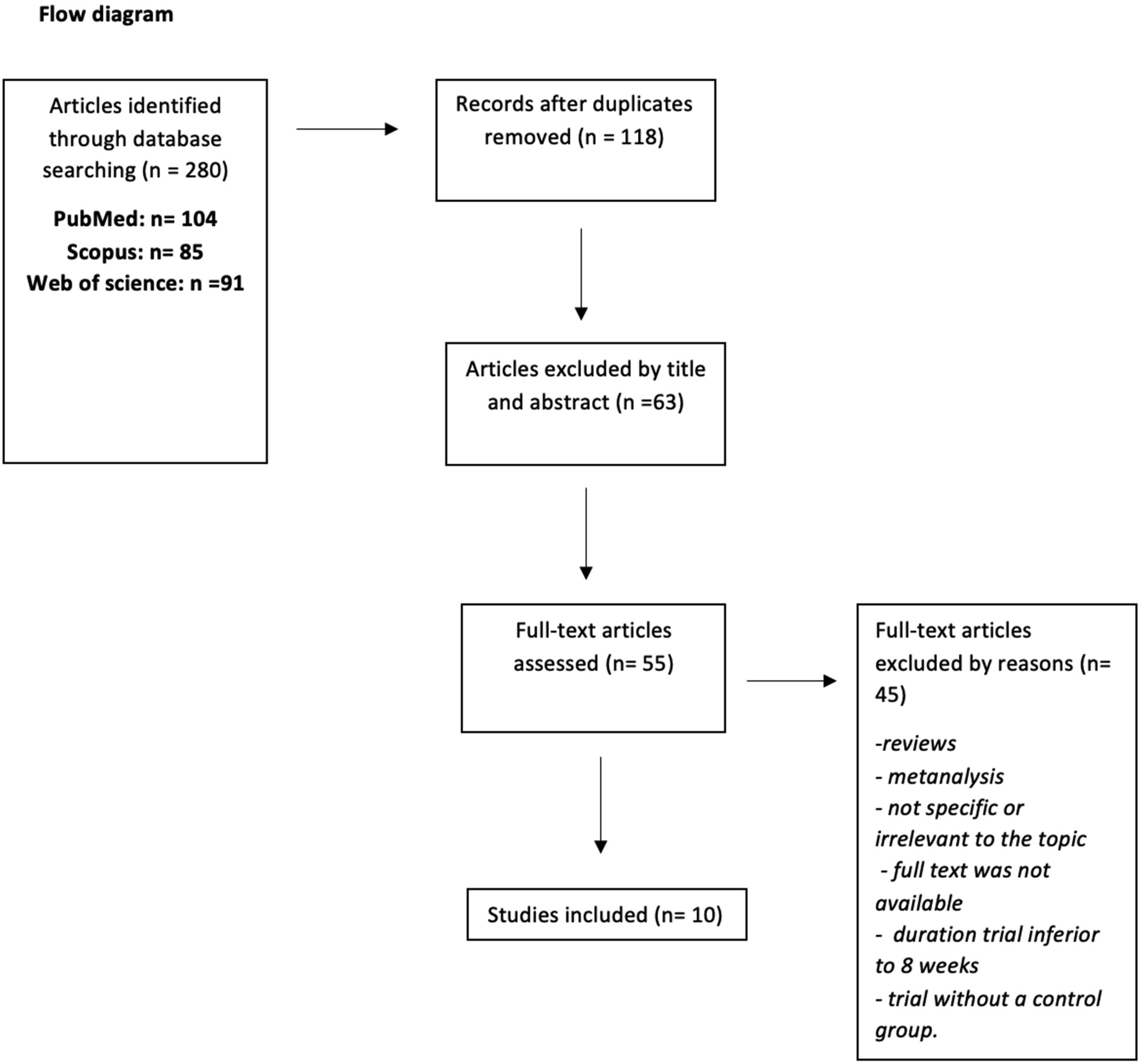
[12] | Page MJ, McKenzie JE, Bossuyt PM, et al. (2021) The PRISMA 2020 statement: an updated guideline for reporting systematic reviews. BMJ : n71. https://doi.org/10.1136/bmj.n71 |
[13] | Abdelrahman AA, Noaman M, Fawzy M, et al. (2021) A double-blind randomized clinical trial of high frequency rTMS over the DLPFC on nicotine dependence, anxiety and depression. Sci Rep 11: 1640. https://doi.org/10.1038/s41598-020-80927-5 |
[14] | Amiaz R, Levy D, Vainiger D, et al. (2009) Repeated high-frequency transcranial magnetic stimulation over the dorsolateral prefrontal cortex reduces cigarette craving and consumption. Addiction 104: 653-660. https://doi.org/10.1111/j.1360-0443.2008.02448.x |
[15] | Li X, Hartwell KJ, Henderson S, et al. (2020) Two weeks of image-guided left dorsolateral prefrontal cortex repetitive transcranial magnetic stimulation improves smoking cessation: A double-blind, sham-controlled, randomized clinical trial. Brain Stimul 13: 1271-1279. https://doi.org/10.1016/j.brs.2020.06.007 |
[16] | Sheffer CE, Bickel WK, Brandon TH, et al. (2018) Preventing relapse to smoking with transcranial magnetic stimulation: Feasibility and potential efficacy. Drug Alcohol Depend 182: 8-18. https://doi.org/10.1016/j.drugalcdep.2017.09.037 |
[17] | Trojak B, Meille V, Achab S, et al. (2015) Transcranial Magnetic Stimulation Combined With Nicotine Replacement Therapy for Smoking Cessation: A Randomized Controlled Trial. Brain Stimul 8: 1168-1174. https://doi.org/10.1016/j.brs.2015.06.004 |
[18] | Dieler AC, Dresler T, Joachim K, et al. (2014) Can Intermittent Theta Burst Stimulation as Add-On to Psychotherapy Improve Nicotine Abstinence? Results from a Pilot Study. Eur Addict Res 20: 248-253. https://doi.org/10.1159/000357941 |
[19] | Dinur-Klein L, Dannon P, Hadar A, et al. (2014) Smoking Cessation Induced by Deep Repetitive Transcranial Magnetic Stimulation of the Prefrontal and Insular Cortices: A Prospective, Randomized Controlled Trial. Biol Psychiatry 76: 742-749. https://doi.org/10.1016/j.biopsych.2014.05.020 |
[20] | Zangen A, Moshe H, Martinez D, et al. (2021) Repetitive transcranial magnetic stimulation for smoking cessation: a pivotal multicenter double-blind randomized controlled trial. World Psychiatry 20: 397-404. https://doi.org/10.1002/wps.20905 |
[21] | Ibrahim C, Tang VM, Blumberger DM, et al. (2023) Efficacy of insula deep repetitive transcranial magnetic stimulation combined with varenicline for smoking cessation: A randomized, double-blind, sham controlled trial. Brain Stimul 16: 1501-1509. https://doi.org/10.1016/j.brs.2023.10.002 |
[22] | Ghorbani Behnam S, Mousavi SA, Emamian MH (2019) The effects of transcranial direct current stimulation compared to standard bupropion for the treatment of tobacco dependence: A randomized sham-controlled trial. Eur Psychiat 60: 41-48. https://doi.org/10.1016/j.eurpsy.2019.04.010 |
[23] | Tseng P, Jeng J, Zeng B, et al. (2022) Efficacy of non-invasive brain stimulation interventions in reducing smoking frequency in patients with nicotine dependence: a systematic review and network meta-analysis of randomized controlled trials. Addiction 117: 1830-1842. https://doi.org/10.1111/add.15624 |
[24] | Petit B, Dornier A, Meille V, et al. (2022) Non-invasive brain stimulation for smoking cessation: a systematic review and meta-analysis. Addiction 117: 2768-2779. https://doi.org/10.1111/add.15889 |
[25] | Lefaucheur J-P, Aleman A, Baeken C, et al. (2020) Evidence-based guidelines on the therapeutic use of repetitive transcranial magnetic stimulation (rTMS): An update (2014–2018). Clin Neurophysiol 131: 474-528. https://doi.org/10.1016/j.clinph.2019.11.002 |
[26] | Lefaucheur J-P, André-Obadia N, Antal A, et al. (2014) Evidence-based guidelines on the therapeutic use of repetitive transcranial magnetic stimulation (rTMS). Clin Neurophysiol 125: 2150-2206. https://doi.org/10.1016/j.clinph.2014.05.021 |
[27] | Mahoney JJ, Hanlon CA, Marshalek PJ, et al. (2020) Transcranial magnetic stimulation, deep brain stimulation, and other forms of neuromodulation for substance use disorders: Review of modalities and implications for treatment. J Neurol Sci 418: 117149. https://doi.org/10.1016/j.jns.2020.117149 |
[28] | Liu Q, Yuan T (2021) Noninvasive brain stimulation of addiction: one target for all?. Psychoradiology 1: 172-184. https://doi.org/10.1093/psyrad/kkab016 |
[29] | Kang N, Kim RK, Kim HJ (2019) Effects of transcranial direct current stimulation on symptoms of nicotine dependence: A systematic review and meta-analysis. Addict Behav 96: 133-139. https://doi.org/10.1016/j.addbeh.2019.05.006 |
[30] | Watson NL, Carpenter MJ, Saladin ME, et al. (2010) Evidence for greater cue reactivity among low-dependent vs. high-dependent smokers. Addict Behav 35: 673-677. https://doi.org/10.1016/j.addbeh.2010.02.010 |
[31] | Kim W-S, Paik N-J (2021) Safety Review for Clinical Application of Repetitive Transcranial Magnetic Stimulation. Brain Neurorehabilitation 14. https://doi.org/10.12786/bn.2021.14.e6 |
[32] | Mattioli F, Maglianella V, D'Antonio S, et al. (2024) Non-invasive brain stimulation for patients and healthy subjects: Current challenges and future perspectives. J Neurol Sci 456: 122825. https://doi.org/10.1016/j.jns.2023.122825 |
[33] | Wessel MJ, Egger P, Hummel FC (2021) Predictive models for response to non-invasive brain stimulation in stroke: A critical review of opportunities and pitfalls. Brain Stimul 14: 1456-1466. https://doi.org/10.1016/j.brs.2021.09.006 |
Parameters | Biological meanings |
p | The proportion of population that get vaccinated immediately after birth |
u1 | Vaccinated rate |
β | Per capita transmission coefficient |
μ | Per capita natural death rate / birth rate |
α | Per capita recovery rate |
σ | The intensities of the white noise |
S(t) | Susceptible proportion in the total population |
I(t) | Infected proportion in the total population |
V(t) | Vaccinated proportion in the total population |