Human and animal diseases have always been reported to be treated by medicinal herbs owing to their constituents. Excess sodium metavanadate is a potential environmental toxin when consumed and could induce oxidative damage leading to various neurological disorders and Parkinsons-like diseases. This study is designed to investigate the impact of the flavonoid Glycoside Fraction of Ginkgo Biloba Extract (GBE) (at 30 mg/kg body weight) on vanadium-treated rats. Animals were divided randomly into four groups: Control (Ctrl, normal saline), Ginkgo Biloba (GIBI, 30mg/kg BWT), Vanadium (VANA, 10 mg/kg BWT) and Vanadium + Ginkgo biloba (VANA + GIBI). Markers of oxidative stress (Glutathione Peroxidase and Catalase) were assessed and found to be statistically increased with GIBI when compared with CTRL and treatment groups. Results from routine staining revealed that the control and GIBI group had a normal distribution of cells and a pronounced increase in cell count respectively compared to the VANA group. When compared to the VANA group, the NeuN photomicrographs revealed that the levels of GIBI were within the normal range (***p < 0.001; ** p < 001). The treatment with GIBI showed a better response by increasing the neuronal cells in the VANA+GIBI when compared with the VANA group. The NLRP3 Inflammasome photomicrographs denoted that there was a decrease in NLRP3-positive cells in the control and GIBI groups. The treatment group shows fewer cells compared to that of the VANA group. The treatment group shows fewer cells compared to that of the VANA group. The findings of the study confirmed that ginkgo biloba extract via its flavonoid glycoside fraction has favorable impacts in modulating vanadium-induced brain damage with the potential ability to lower antioxidant levels and reduce neuroinflammation.
Citation: Adeshina O. Adekeye, Adedamola A. Fafure, Morayo M. Omodele, Lawrence D. Adedayo, Victor O. Ekundina, Damilare A. Adekomi, Ephraim Samuel Jen, Thomas K. Adenowo. Flavonoid glycoside fraction of Ginkgo biloba extract modulates antioxidants imbalance in vanadium-induced brain damage[J]. AIMS Neuroscience, 2023, 10(2): 178-189. doi: 10.3934/Neuroscience.2023015
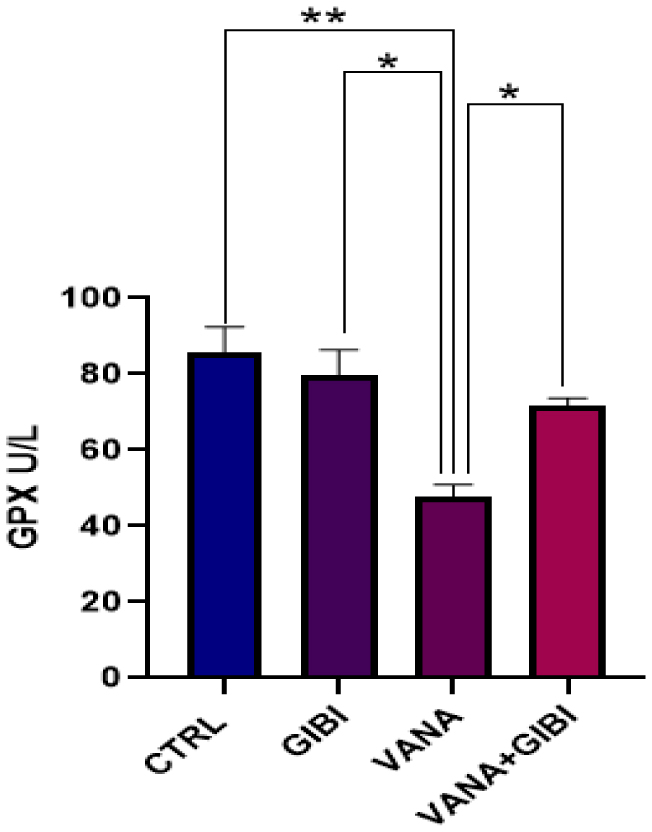
Human and animal diseases have always been reported to be treated by medicinal herbs owing to their constituents. Excess sodium metavanadate is a potential environmental toxin when consumed and could induce oxidative damage leading to various neurological disorders and Parkinsons-like diseases. This study is designed to investigate the impact of the flavonoid Glycoside Fraction of Ginkgo Biloba Extract (GBE) (at 30 mg/kg body weight) on vanadium-treated rats. Animals were divided randomly into four groups: Control (Ctrl, normal saline), Ginkgo Biloba (GIBI, 30mg/kg BWT), Vanadium (VANA, 10 mg/kg BWT) and Vanadium + Ginkgo biloba (VANA + GIBI). Markers of oxidative stress (Glutathione Peroxidase and Catalase) were assessed and found to be statistically increased with GIBI when compared with CTRL and treatment groups. Results from routine staining revealed that the control and GIBI group had a normal distribution of cells and a pronounced increase in cell count respectively compared to the VANA group. When compared to the VANA group, the NeuN photomicrographs revealed that the levels of GIBI were within the normal range (***p < 0.001; ** p < 001). The treatment with GIBI showed a better response by increasing the neuronal cells in the VANA+GIBI when compared with the VANA group. The NLRP3 Inflammasome photomicrographs denoted that there was a decrease in NLRP3-positive cells in the control and GIBI groups. The treatment group shows fewer cells compared to that of the VANA group. The treatment group shows fewer cells compared to that of the VANA group. The findings of the study confirmed that ginkgo biloba extract via its flavonoid glycoside fraction has favorable impacts in modulating vanadium-induced brain damage with the potential ability to lower antioxidant levels and reduce neuroinflammation.

| [1] |
Blauwendraat C, Nalls MA, Singleton AB (2020) The genetic architecture of Parkinson's disease. Lancet Neurol 19: 170-178. https://doi.org/10.1016/S1474-4422(19)30287-X 
|
| [2] |
Adekeye AO, Irawo-Joseph G, Fafure AA (2020) Ficus exasperate vahl leaves extract attenuates motor deficit in vanadium-induced parkinsonism mice. Anat Cell Biol 53: e10. https://doi.org/10.5115/acb.19.205
|
| [3] |
Adekeye AO, Adefule AK, Shallie P, et al. (2018) Cholecalciferol Attenuates 1-Methyl-4-Phenyl-1,2,3,6-Tetrahydropyridine-Induced Parkinson's Like-Disease Variation in Oxidative Stress Markers, Mouse Behaviour and Cellular morphology of Striatum and Substantia nigra. Anat J Africa 7: 1258-1274. https://doi.org/10.1016/j.ibror.2019.09.044
|
| [4] | Berkovits M, Farrar J (2010) Conflicting emotions: The connection between affective perspective taking and theory of mind. Brit J Dev Psyschol 24: 401-418. https://doi.org/10.1348/026151005X50302 |
| [5] |
Han W, Ahn D, Kim S, et al. (2018) Psychiatric Manifestation in Patients with Parkinson's Disease. J Korean MedSci 33: e300. https://doi.org/10.3346/jkms.2018.33.e300
|
| [6] |
Simon DK, Tanner CM, Brundin P (2020) ParkinsonDiseaseEpidemiology, Pathology, Genetics and Pathophysiology. Clin Geriatr Med 36: 1-12. https://doi.org/10.1016/j.cger.2019.08.002
|
| [7] | Antrekowitsch H, Luidold S, Gaugl H Thermodynamic Calculations of the Production of Ferrovanadium from V-containing Steelworks Slags with a low Content of V2O5.Part 1 (2021). |
| [8] |
Li H-Y, Fang H-X, Wang K, et al. (2015) Asynchronous extraction of vanadium and chromium from vanadium slag by stepwise sodium roasting–water leaching. Hydrometallurgy 156: 124-135. https://doi.org/10.1016/j.hydromet.2015.06.003
|
| [9] | Zou K, Junhu X, Guanjie L, et al. (2021) Effective Extraction of Vanadium from Bauxite-Type Vanadium Ore Using Roasting and Leaching. J Metals 11: 9. https://doi.org/10.3390/met11091342 |
| [10] | Tiwari AK (2004) Antioxidants: New generation therapeutic base for treatment of polygenic disorders. Curr Sci 86: 1092-102. |
| [11] |
Tang L, Su Y, He J, et al. (2012) Urinary Titanium and Vanadium and Breast Cancer: A Case-Control Study. Nutr Cancer 64: 368-376. https://doi.org/10.1080/01635581.2012.654586
|
| [12] |
Isah T (2015) Rethinking Ginkgo biloba L.: Medicinal uses and conservation. Pharmacognosy Rev 9: 140. https://doi.org/10.4103/0973-7847.162137
|
| [13] |
Mei N, Guo X, Ren Z, et al. (2017) Review of Ginkgo biloba-induced toxicity, from experimental studies to human case reports. J Environ Sci Health C Environ Carcinog Ecotoxicol Rev 35: 1-28. https://doi.org/10.1080/10590501.2016.1278298
|
| [14] |
Zhang Q, Wang G, Ji-ye A, et al. (2009) Application of GC/MS-based metabonomic profiling in studying the lipid-regulating effects of Ginkgo biloba extract on diet-induced hyperlipidemia in rats. Acta Pharmacologica Sinica 30: 1674-1687. https://doi.org/10.1038/aps.2009.173
|
| [15] | Paglia DE, Valentine WN (1967) Studies on the quantitative and qualitative characterization of erythrocyte glutathione peroxidase. J Lab Clin Med 70: 158-169. |
| [16] | Koroliuk MA, Ivanova IG, Maiorova (1988) A method of determining catalase activity. LaboratornoeDelo 1: 16-19. |
| [17] |
Benzie IF, Strain JJ (1996) The ferric reducing ability of plasma (FRAP) as a measure of antioxidant power. FRAP Assay Anal Biochem 239: 70-76. https://doi.org/10.1006/abio.1996.0292
|
| [18] |
Adekeye AO, Fafure AA, Ogunsemowo AE, et al. (2022) Naringin ameliorates motor dysfunction and exerts neuroprotective role against vanadium-induced neurotoxicity. AIMS Neurosci 9: 536-550. https://doi.org/10.3934/Neuroscience.2022031
|
| [19] |
Preiser JC (2012) Oxidative Stress. Jpen Parenter Enter 36: 147-15. https://doi.org/10.1177/0148607111434963
|
| [20] |
Muller L, Lustgarten S, Jang Y, et al. (2007) Trends in oxidative aging theories. Free Radical Bio Med 43: 477503. https://doi.org/10.1016/j.freeradbiomed.2007.03.034
|
| [21] |
Afeseh Ngwa H, Kanthasamy A, Anantharam V, et al. (2009) Vanadium induces dopaminergic neurotoxicity via protein kinase Cdeltadependent oxidative signaling mechanisms: relevance to etiopathogenesis of Parkinson's disease. Toxicol Apply Pharmacol 240: 273-85. https://doi.org/10.1016/j.taap.2009.07.025
|
| [22] |
Kim J, Basak JM, Holtzman DM (2009) The role of apolipoprotein E in Alzheimer's disease. Neuron 63: 287-303. https://doi.org/10.1016/j.neuron.2009.06.026
|
| [23] |
Fatola OI, Olaolorun FA, Olopade FE, et al. (2018) Trends in vanadium neurotoxicity. Brain Res Bull 145: 75-80. https://doi.org/10.1016/j.brainresbull.2018.03.010
|
| [24] |
Mariathasan S, Newton K, Monack DM, et al. (2004) Differential activation of the inflammasome by caspase-1 adaptors ASC and Ipaf. Nature 430: 213-218. https://doi.org/10.1038/nature02664
|
| [25] |
Fafure AA, Adekeye AO, Enye LA, et al. (2018) Ficus ExasperataVahl improves manganese-induced neurotoxicity and motor dysfunction in mice. Anat J Africa 7: 1206-1219. https://doi.org/10.4314/aja.v7i2.174140
|
| [26] |
Folarin OR, Snyder AM, Peters DG, et al. (2017) Brain metal distribution and neuro-inflammatory profiles after chronic vanadium administration and withdrawal in mice. Front Neuroanat 11: 58. https://doi.org/10.3389/fnana.2017.00058
|
| [27] | Brondino N, De Silvestri A, Re S, et al. (2013) A Systematic Review and Meta-Analysis of Ginkgo biloba in Neuropsychiatric Disorders: From Ancient Tradition to Modern-Day Medicine. Evid Based Compl Alt . https://doi.org/10.1155/2013/915691 |


Figures(5)

Adeshina O. Adekeye, Adedamola A. Fafure, Morayo M. Omodele, Lawrence D. Adedayo, Victor O. Ekundina, Damilare A. Adekomi, Ephraim Samuel Jen, Thomas K. Adenowo. Flavonoid glycoside fraction of Ginkgo biloba extract modulates antioxidants imbalance in vanadium-induced brain damage[J]. AIMS Neuroscience, 2023, 10(2): 178-189. doi: 10.3934/Neuroscience.2023015


 DownLoad: