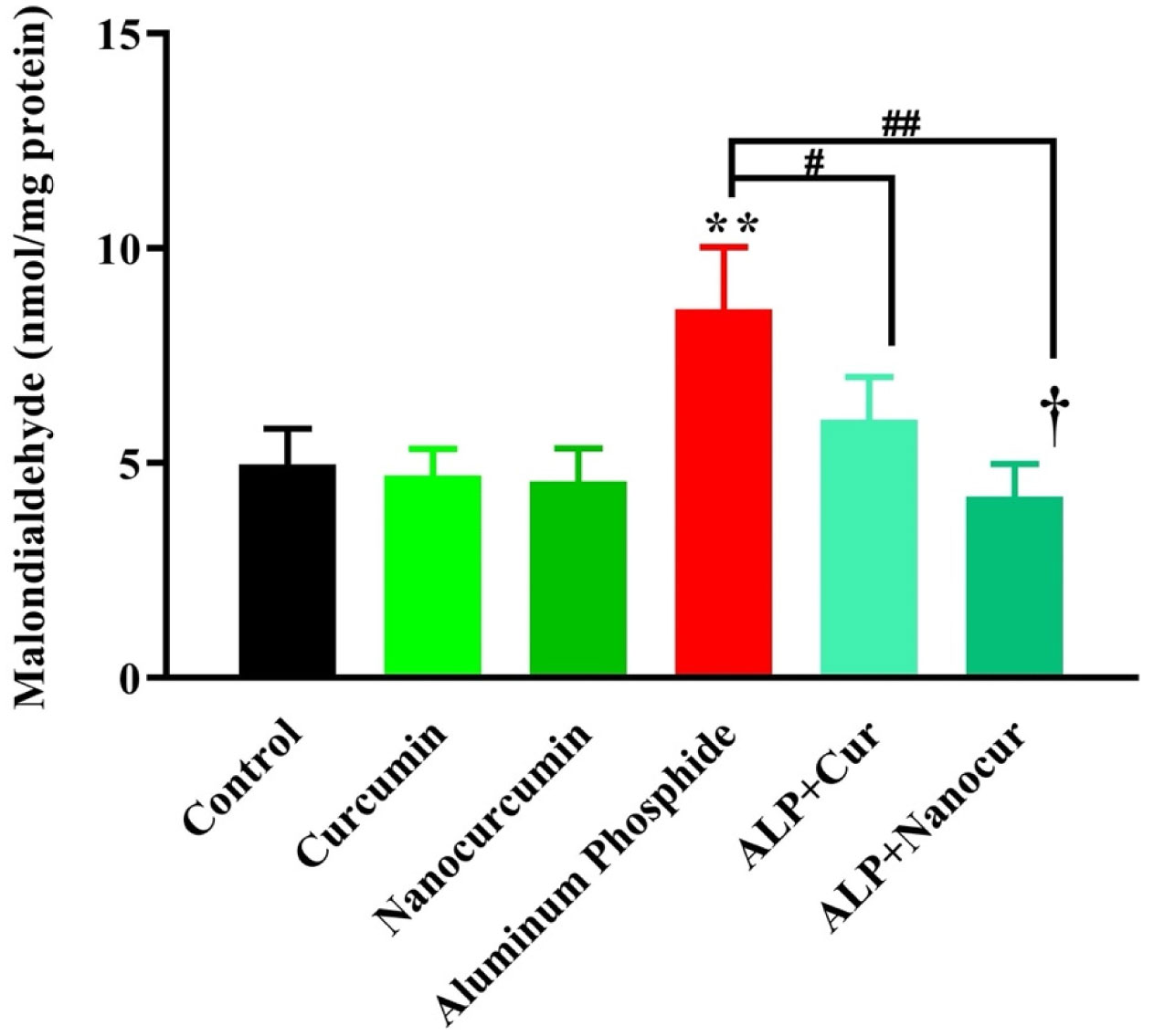
Aluminum phosphide (ALP) is among the most significant causes of brain toxicity and death in many countries. Curcumin (CUR), a major turmeric component, is a potent protective agent against many diseases, including brain toxicity. This study aimed to examine the probable protection potential of nanomicelle curcumin (nanomicelle-CUR) and its underlying mechanism in a rat model of ALP-induced brain toxicity. A total of 36 Wistar rats were randomly divided into six groups (n = 6) and exposed to ALP (2 mg/kg/day, orally) + CUR or nanomicelle-CUR (100 mg/kg/day, orally) for 7 days. Then, they were anesthetized, and brain tissue samples were dissected to evaluate histopathological alterations, oxidative stress biomarkers, gene expression of SIRT1, FOXO1a, FOXO3a, CAT and GPX in brain tissue via hematoxylin and eosin (H&E) staining, biochemical and enzyme-linked immunosorbent assay (ELISA) methods and Real-Time PCR analysis. CUR and nanomicelle-CUR caused significant improvement in ALP-induced brain damage by reducing the MDA levels and induction of antioxidant capacity (TTG, TAC and SOD levels) and antioxidant enzymes (CAT, GPX), modulation of histopathological changes and up-regulation of gene expression of SIRT1 in brain tissue. It was concluded that nanomicelle-CUR treatment ameliorated the harmful effects of ALP-induced brain toxicity by reducing oxidative stress. Therefore, it could be considered a suitable therapeutic choice for ALP poisoning.
Citation: Milad Khodavysi, Nejat Kheiripour, Hassan Ghasemi, Sara Soleimani-Asl, Ali Fathi Jouzdani, Mohammadmahdi Sabahi, Zahra Ganji, Zahra Azizi, Akram Ranjbar. How can nanomicelle-curcumin modulate aluminum phosphide-induced neurotoxicity?: Role of SIRT1/FOXO3 signaling pathway[J]. AIMS Neuroscience, 2023, 10(1): 56-74. doi: 10.3934/Neuroscience.2023005
Aluminum phosphide (ALP) is among the most significant causes of brain toxicity and death in many countries. Curcumin (CUR), a major turmeric component, is a potent protective agent against many diseases, including brain toxicity. This study aimed to examine the probable protection potential of nanomicelle curcumin (nanomicelle-CUR) and its underlying mechanism in a rat model of ALP-induced brain toxicity. A total of 36 Wistar rats were randomly divided into six groups (n = 6) and exposed to ALP (2 mg/kg/day, orally) + CUR or nanomicelle-CUR (100 mg/kg/day, orally) for 7 days. Then, they were anesthetized, and brain tissue samples were dissected to evaluate histopathological alterations, oxidative stress biomarkers, gene expression of SIRT1, FOXO1a, FOXO3a, CAT and GPX in brain tissue via hematoxylin and eosin (H&E) staining, biochemical and enzyme-linked immunosorbent assay (ELISA) methods and Real-Time PCR analysis. CUR and nanomicelle-CUR caused significant improvement in ALP-induced brain damage by reducing the MDA levels and induction of antioxidant capacity (TTG, TAC and SOD levels) and antioxidant enzymes (CAT, GPX), modulation of histopathological changes and up-regulation of gene expression of SIRT1 in brain tissue. It was concluded that nanomicelle-CUR treatment ameliorated the harmful effects of ALP-induced brain toxicity by reducing oxidative stress. Therefore, it could be considered a suitable therapeutic choice for ALP poisoning.

| [1] | Ranjbar A, Gholami L, Ghasemi H, et al. (2020) EEffects of nano-curcumin and curcumin on the oxidant and antioxidant system of the liver mitochondria in aluminum phosphide-induced experimental toxicity. Nanomed J 7: 58-64. |
| [2] |
Kariman H, Heydari K, Fakhri M, et al. (2012) Aluminium phosphide poisoning and oxidative stress. J Med Toxicol 8: 281-284. https://doi.org/10.1007/s13181-012-0219-1 
|
| [3] |
Meena MC, Mittal S, Rani Y (2015) Fatal aluminium phosphide poisoning. Interdisciplinary toxicology 8: 65-67. https://doi.org/10.1515/intox-2015-0010
|
| [4] | Hashemi-Domeneh B, Zamani N, Hassanian-Moghaddam H, et al. (2016) A review of aluminium phosphide poisoning and a flowchart to treat it. Arch Ind Hyg Toxicol 67: 183-193. https://doi.org/10.1515/aiht-2016-67-2784 |
| [5] |
Arora V, Gupta V (2017) Criminal Poisoning with Aluminium Phosphide. J Punjab Acad Forensic Med Toxicol 17: 94-95. https://doi.org/10.5958/0974-083X.2017.00020.6
|
| [6] |
Gouda AS, El-Nabarawy NA, Ibrahim SF (2018) Moringa oleifera extract (Lam) attenuates Aluminium phosphide-induced acute cardiac toxicity in rats. Toxicol Rep 5: 209-212. https://doi.org/10.1016/j.toxrep.2018.01.001
|
| [7] |
Tripathi S, Pandey S (2007) The effect of aluminium phosphide on the human brain: a histological study. Med Sci Law 47: 141-146. https://doi.org/10.1258/rsmmsl.47.2.141
|
| [8] |
Dua R, Gill KD (2001) Aluminium phosphide exposure: implications on rat brain lipid peroxidation and antioxidant defence system. Pharmacol Toxico 89: 315-319. https://doi.org/10.1034/j.1600-0773.2001.d01-167.x
|
| [9] | Odo G, Agwu E, Ossai N, et al. (2017) Effects of Aluminium Phosphide on the Behaviour, Haematology, Oxidative Stress Biomarkers and Biochemistry of African Catfish (Clarias gariepinus) Juvenile. Pak J Zool 49: 433-444. https://doi.org/10.17582/journal.pjz/2017.49.2.405.415 |
| [10] | Fakhraei N, Hashemibakhsh R, Rezayat SM, et al. (2019) On the Benefit of Nanocurcumin on Aluminium Phosphide-induced Cardiotoxicity in a Rat Model. Nanomed Res J 4: 111-121. |
| [11] |
Dai C, Ciccotosto GD, Cappai R, et al. (2018) Curcumin attenuates colistin-induced neurotoxicity in N2a cells via anti-inflammatory activity, suppression of oxidative stress, and apoptosis. Mol Neurobiol 55: 421-434. https://doi.org/10.1007/s12035-016-0276-6
|
| [12] | Malhotra SK, Mandal T (2017) A REVIEW OF THERAPEUTIC EFFECTS OF CURCUMIN'S BASED ON ITS ANTI-INFLAMMATORY PROPERTIES AND ANTICANCER ACTIVITIES IN UTTARAKHAND. ENVIS Bulletin Himalayan Ecology 25: 57. |
| [13] |
Gupta N, Verma K, Nalla S, et al. (2020) Free Radicals as a Double-Edged Sword: The Cancer Preventive and Therapeutic Roles of Curcumin. Molecules (Basel, Switzerland) 25: 5390. https://doi.org/10.3390/molecules25225390
|
| [14] |
Mendoza-Magaña ML, Espinoza-Gutiérrez HA, Nery-Flores SD, et al. (2021) Curcumin Decreases Hippocampal Neurodegeneration and Nitro-Oxidative Damage to Plasma Proteins and Lipids Caused by Short-Term Exposure to Ozone. Molecules 26: 4075. https://doi.org/10.3390/molecules26134075
|
| [15] | Borra SK, Mahendra J, Gurumurthy P (2014) Effect of curcumin against oxidation of biomolecules by hydroxyl radicals. J Clin Diagn Res JCDR 8: CC01. https://doi.org/10.7860/JCDR/2014/8517.4967 |
| [16] |
Sharma D, Sethi P, Hussain E, et al. (2009) Curcumin counteracts the aluminium-induced ageing-related alterations in oxidative stress, Na+, K+ ATPase and protein kinase C in adult and old rat brain regions. Biogerontology 10: 489-502. https://doi.org/10.1007/s10522-008-9195-x
|
| [17] |
Mahaki H, Tanzadehpanah H, Abou-Zied OK, et al. (2019) Cytotoxicity and antioxidant activity of Kamolonol acetate from Ferula pseudalliacea, and studying its interactions with calf thymus DNA (ct-DNA) and human serum albumin (HSA) by spectroscopic and molecular docking techniques. Process Biochem 79: 203-213. https://doi.org/10.1016/j.procbio.2018.12.004
|
| [18] |
Moghadam NH, Salehzadeh S, Rakhtshah J, et al. (2019) Preparation of a highly stable drug carrier by efficient immobilization of human serum albumin (HSA) on drug-loaded magnetic iron oxide nanoparticles. Int J Biol Macromol 125: 931-940. https://doi.org/10.1016/j.ijbiomac.2018.12.143
|
| [19] |
Tanzadehpanah H, Mahaki H, Moradi M, et al. (2018) Human serum albumin binding and synergistic effects of gefitinib in combination with regorafenib on colorectal cancer cell lines. Colorectal Cancer 7: CRC03. https://doi.org/10.2217/crc-2017-0018
|
| [20] |
Singh DV, Bharti SK, Agarwal S, et al. (2014) Study of interaction of human serum albumin with curcumin by NMR and docking. J Mol Model 20: 2365. https://doi.org/10.1007/s00894-014-2365-7
|
| [21] |
Tonnesen H, Karlsen J (1985) Studies on curcumin and curcuminoids. V. Alkaline degradation of curcumin. Zeitschrift für Lebensmittel-Untersuchung und-Forschung 180: 132-134. https://doi.org/10.1007/BF01042637
|
| [22] |
Kaminaga Y, Nagatsu A, Akiyama T, et al. (2003) Production of unnatural glucosides of curcumin with drastically enhanced water solubility by cell suspension cultures of Catharanthus roseus. FEBS Lett 555: 311-316. https://doi.org/10.1016/S0014-5793(03)01265-1
|
| [23] |
Hussain Z, Thu HE, Amjad MW, et al. (2017) Exploring recent developments to improve antioxidant, anti-inflammatory and antimicrobial efficacy of curcumin: A review of new trends and future perspectives. Mat Sci Eng C 77: 1316-1326. https://doi.org/10.1016/j.msec.2017.03.226
|
| [24] |
Karthikeyan A, Senthil N, Min T (2020) Nanocurcumin: A promising candidate for therapeutic applications. Front Pharmacol 11. https://doi.org/10.3389/fphar.2020.00487
|
| [25] |
Hosseini A, Rasaie D, Soleymani Asl S, et al. (2019) Evaluation of the protective effects of curcumin and nanocurcumin against lung injury induced by sub-acute exposure to paraquat in rats. Toxin Rev 40: 1233-1241. https://doi.org/10.1080/15569543.2019.1675707
|
| [26] |
Peer D, Karp JM, Hong S, et al. (2007) Nanocarriers as an emerging platform for cancer therapy. Nat Nanotechnol 2: 751-760. https://doi.org/10.1038/nnano.2007.387
|
| [27] |
Mishra D, Hubenak JR, Mathur AB (2013) Nanoparticle systems as tools to improve drug delivery and therapeutic efficacy. J Biomed Mater Res A 101: 3646-3660. https://doi.org/10.1002/jbm.a.34642
|
| [28] |
Jones CG, Daniel Hare J, Compton SJ (1989) Measuring plant protein with the Bradford assay: 1. Evaluation and standard method. J Chem Ecol 15: 979-992. https://doi.org/10.1007/BF01015193
|
| [29] |
Ohkawa H, Ohishi N, Yagi K (1979) Assay for lipid peroxides in animal tissues by thiobarbituric acid reaction. Anal Biochem 95: 351-358. https://doi.org/10.1016/0003-2697(79)90738-3
|
| [30] |
Rao B, Simpson C, Lin H, et al. (2014) Determination of thiol functional groups on bacteria and natural organic matter in environmental systems. Talanta 119: 240-247. https://doi.org/10.1016/j.talanta.2013.11.004
|
| [31] |
Benzie IF, Szeto Y (1999) Total antioxidant capacity of teas by the ferric reducing/antioxidant power assay. J Agric Food Chem 47: 633-636. https://doi.org/10.1021/jf9807768
|
| [32] |
Mariani E, Polidori M, Cherubini A, et al. (2005) Oxidative stress in brain aging, neurodegenerative and vascular diseases: an overview. J Chromatogr B 827: 65-75. https://doi.org/10.1016/j.jchromb.2005.04.023
|
| [33] |
Love S (1999) Oxidative stress in brain ischemia. Brain Pathol 9: 119-131. https://doi.org/10.1111/j.1750-3639.1999.tb00214.x
|
| [34] |
Yang Q, Huang Q, Hu Z, et al. (2019) Potential neuroprotective treatment of stroke: targeting excitotoxicity, oxidative stress, and inflammation. Front Neurosci 13: 1036. https://doi.org/10.3389/fnins.2019.01036
|
| [35] |
Praticò D, Clark CM, Liun F, et al. (2002) Increase of brain oxidative stress in mild cognitive impairment: a possible predictor of Alzheimer disease. Arch Neurol 59: 972-976. https://doi.org/10.1001/archneur.59.6.972
|
| [36] |
Sawa A, Sedlak TW (2016) Oxidative stress and inflammation in schizophrenia. Schizophr Res 176: 1-2. https://doi.org/10.1016/j.schres.2016.06.014
|
| [37] |
Sciuto AM, Wong BJ, Martens ME, et al. (2016) Phosphine toxicity: a story of disrupted mitochondrial metabolism. Ann N Y Acad Sci 1374: 41. https://doi.org/10.1111/nyas.13081
|
| [38] |
López-Posadas R, González R, Ballester I, et al. (2011) Tissue-nonspecific alkaline phosphatase is activated in enterocytes by oxidative stress via changes in glycosylation. Inflamm Bowel Dis 17: 543-556. https://doi.org/10.1002/ibd.21381
|
| [39] |
Uttara B, Singh AV, Zamboni P, et al. (2009) Oxidative stress and neurodegenerative diseases: a review of upstream and downstream antioxidant therapeutic options. Curr Neuropharmacol 7: 65-74. https://doi.org/10.2174/157015909787602823
|
| [40] |
Bakacak M, Kılınç M, Serin S, et al. (2015) Changes in copper, zinc, and malondialdehyde levels and superoxide dismutase activities in pre-eclamptic pregnancies. Med Sci Monit 21: 2414-2420. https://doi.org/10.12659/MSM.895002
|
| [41] | Aziz IA, Yacoub M, Rashid L, et al. (2015) Malondialdehyde; Lipid peroxidation plasma biomarker correlated with hepatic fibrosis in human Schistosoma mansoni infection. Acta Parasitol 60: 735-742. https://doi.org/10.1515/ap-2015-0105 |
| [42] | Afolabi OK, Oyewo EB, Adeleke GE, et al. (2019) Mitigation of Aluminium Phosphide-induced Hematotoxicity and Ovarian Oxidative Damage in Wistar Rats by Hesperidin. Am J Biochem 9: 7-16. |
| [43] |
Tehrani H, Halvaie Z, Shadnia S, et al. (2013) Protective effects of N-acetylcysteine on aluminum phosphide-induced oxidative stress in acute human poisoning. Clin Toxicol 51: 23-28. https://doi.org/10.3109/15563650.2012.743029
|
| [44] |
Dinc M, Ulusoy S, Is A, et al. (2016) Thiol/disulphide homeostasis as a novel indicator of oxidative stress in sudden sensorineural hearing loss. J Laryngol Otol 130: 447-452. https://doi.org/10.1017/S002221511600092X
|
| [45] |
Suresh D, Annam V, Pratibha K, et al. (2009) Total antioxidant capacity–a novel early bio-chemical marker of oxidative stress in HIV infected individuals. J Biomed Sci 16: 61. https://doi.org/10.1186/1423-0127-16-61
|
| [46] | Afolabi OK, Wusu AD, Ugbaja R, et al. (2018) Aluminium phosphide-induced testicular toxicity through oxidative stress in Wistar rats: Ameliorative role of hesperidin. Toxicol Res Appl 2: 2397847318812794. https://doi.org/10.1177/2397847318812794 |
| [47] |
Ciftci O, Turkmen NB, Taslıdere A (2018) Curcumin protects heart tissue against irinotecan-induced damage in terms of cytokine level alterations, oxidative stress, and histological damage in rats. N-S Arch Pharmacol 391: 783-791. https://doi.org/10.1007/s00210-018-1495-3
|
| [48] | Rajeswari A (2006) Curcumin protects mouse brain from oxidative stress caused by 1-methyl-4-phenyl-1, 2, 3, 6-tetrahydro pyridine. Eur Rev Med Pharmacol Sci 10: 157. |
| [49] |
Liu J, Gong Z, Wu J, et al. (2021) Hypoxic postconditioning-induced neuroprotection increases neuronal autophagy via activation of the SIRT1/FoxO1 signaling pathway in rats with global cerebral ischemia. Exp Ther Med 22: 695. https://doi.org/10.3892/etm.2021.10127
|
| [50] |
Li XH, Chen C, Tu Y, et al. (2013) Sirt1 promotes axonogenesis by deacetylation of Akt and inactivation of GSK3. Mol Neurobiol 48: 490-499. https://doi.org/10.1007/s12035-013-8437-3
|
| [51] |
Codocedo JF, Allard C, Godoy JA, et al. (2012) SIRT1 regulates dendritic development in hippocampal neurons. PLoS One 7: e47073. https://doi.org/10.1371/journal.pone.0047073
|
| [52] |
Rafalski VA, Ho PP, Brett JO, et al. (2013) Expansion of oligodendrocyte progenitor cells following SIRT1 inactivation in the adult brain. Nat Cell Biol 15: 614-624. https://doi.org/10.1038/ncb2735
|
| [53] | Zhang W, Huang Q, Zeng Z, et al. (2017) Sirt1 Inhibits Oxidative Stress in Vascular Endothelial Cells. Oxid Med Cell Longev 2017: 7543973-7543973. https://doi.org/10.1155/2017/7543973 |
| [54] |
Ren Z, He H, Zuo Z, et al. (2019) The role of different SIRT1-mediated signaling pathways in toxic injury. Cell Mol Biol Lett 24: 36. https://doi.org/10.1186/s11658-019-0158-9
|
| [55] |
Jackson BC, Carpenter C, Nebert DW, et al. (2010) Update of human and mouse forkhead box (FOX) gene families. Hum Genomics 4: 345-352. https://doi.org/10.1186/1479-7364-4-5-345
|
| [56] |
Greer EL, Brunet A (2005) FOXO transcription factors at the interface between longevity and tumor suppression. Oncogene 24: 7410-7425. https://doi.org/10.1038/sj.onc.1209086
|
| [57] |
Fasano C, Disciglio V, Bertora S, et al. (2019) FOXO3a from the Nucleus to the Mitochondria: A Round Trip in Cellular Stress Response. Cells 8: 1110. https://doi.org/10.3390/cells8091110
|
| [58] |
Brown AK, Webb AE (2018) Regulation of FOXO Factors in Mammalian Cells. Curr Top Dev Biol 127: 165-192. https://doi.org/10.1016/bs.ctdb.2017.10.006
|
| [59] |
Olmos Y, Sánchez-Gómez FJ, Wild B, et al. (2013) SirT1 regulation of antioxidant genes is dependent on the formation of a FoxO3a/PGC-1α complex. Antioxid Redox Sign 19: 1507-1521. https://doi.org/10.1089/ars.2012.4713
|
| [60] |
Xiong S, Salazar G, Patrushev N, et al. (2011) FoxO1 mediates an autofeedback loop regulating SIRT1 expression. J Biol Chem 286: 5289-5299. https://doi.org/10.1074/jbc.M110.163667
|
| [61] |
Ferguson D, Shao N, Heller E, et al. (2015) SIRT1-FOXO3a regulate cocaine actions in the nucleus accumbens. J Neurosci 35: 3100-3111. https://doi.org/10.1523/JNEUROSCI.4012-14.2015
|
| [62] |
Gómez-Crisóstomo NP, Rodríguez Martínez E, Rivas-Arancibia S (2014) Oxidative Stress Activates the Transcription Factors FoxO 1a and FoxO 3a in the Hippocampus of Rats Exposed to Low Doses of Ozone. Oxid Med Cell Longev 2014: 805764. https://doi.org/10.1155/2014/805764
|
| [63] |
Yang Y, Duan W, Lin Y, et al. (2013) SIRT1 activation by curcumin pretreatment attenuates mitochondrial oxidative damage induced by myocardial ischemia reperfusion injury. Free Radic Biol Med 65: 667-679. https://doi.org/10.1016/j.freeradbiomed.2013.07.007
|
| [64] |
Sun Q, Jia N, Wang W, et al. (2014) Activation of SIRT1 by curcumin blocks the neurotoxicity of amyloid-β25-35 in rat cortical neurons. Biochem Biophys Res Commun 448: 89-94. https://doi.org/10.1016/j.bbrc.2014.04.066
|
| [65] |
Sun Y, Hu X, Hu G, et al. (2015) Curcumin Attenuates Hydrogen Peroxide-Induced Premature Senescence via the Activation of SIRT1 in Human Umbilical Vein Endothelial Cells. Biol Pharm Bull 38: 1134-1141. https://doi.org/10.1248/bpb.b15-00012
|
| [66] |
Iside C, Scafuro M, Nebbioso A, et al. (2020) SIRT1 Activation by Natural Phytochemicals: An Overview. Front Pharmacol 11. https://doi.org/10.3389/fphar.2020.01225
|
| [67] |
Han J, Pan X-Y, Xu Y, et al. (2012) Curcumin induces autophagy to protect vascular endothelial cell survival from oxidative stress damage. Autophagy 8: 812-825. https://doi.org/10.4161/auto.19471
|
| [68] |
Wang M, Jiang S, Zhou L, et al. (2019) Potential Mechanisms of Action of Curcumin for Cancer Prevention: Focus on Cellular Signaling Pathways and miRNAs. Int J Biol Sci 15: 1200-1214. https://doi.org/10.7150/ijbs.33710
|
| [69] |
Fallah M, Moghble N, Javadi I, et al. (2018) Effect of Curcumin and N-Acetylcysteine on Brain Histology and Inflammatory Factors (MMP-2, 9 and TNF-α) in Rats Exposed to Arsenic. Pharm Sci 24: 264. https://doi.org/10.15171/PS.2018.39
|


Figures(7)

Milad Khodavysi, Nejat Kheiripour, Hassan Ghasemi, Sara Soleimani-Asl, Ali Fathi Jouzdani, Mohammadmahdi Sabahi, Zahra Ganji, Zahra Azizi, Akram Ranjbar. How can nanomicelle-curcumin modulate aluminum phosphide-induced neurotoxicity?: Role of SIRT1/FOXO3 signaling pathway[J]. AIMS Neuroscience, 2023, 10(1): 56-74. doi: 10.3934/Neuroscience.2023005


 DownLoad: