Nexus between crude oil prices, clean energy investments, technology companies and energy democracy

Caner Özdurak; Caner Özdurak

doi:10.3934/GF.2021017

Green Finance

2021, Volume 3, Issue 3: 337-350. doi: 10.3934/GF.2021017

Previous Article Next Article

Research article

Nexus between crude oil prices, clean energy investments, technology companies and energy democracy

Caner Özdurak ^,

Financial Economics Department, Yeditepe University, İstanbul, Turkey

Received: 10 June 2021 Accepted: 27 August 2021 Published: 01 September 2021
JEL Codes: G1, G10, C32, Q4

In this study, we examine the nexus between crude oil prices, clean energy investments, technology companies, and energy democracy. Our dataset incorporates four variables which are S & P Global Clean Energy Index (SPClean), Brent crude oil futures (Brent), CBOE Volatility Index (VIX), and NASDAQ 100 Technology Sector (DXNT) daily prices between 2009 and 2021. The novelty of our study is that we included technology development and market fear as important factors and assess their impact on clean energy investments. DCC-GARCH models are utilized to analyze the spillover impact of market fear, oil prices, and technology company stock returns to clean energy investments. According to our findings when oil prices decrease, the volatility index usually responds by increasing which means that the market is afraid of oil price surges. Renewable investments also tend to decrease in that period following the oil price trend. Moreover, a positive relationship between technology stocks and renewable energy stock returns also exists.
- dynamic spillover,
- renewable energy companies,
- fossil-fuel price,
- energy democracy
Citation: Caner Özdurak. Nexus between crude oil prices, clean energy investments, technology companies and energy democracy[J]. Green Finance, 2021, 3(3): 337-350. doi: 10.3934/GF.2021017

Related Papers:

Abstract

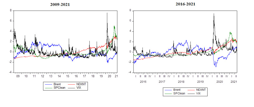
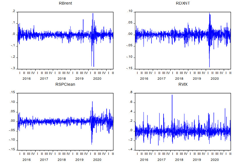
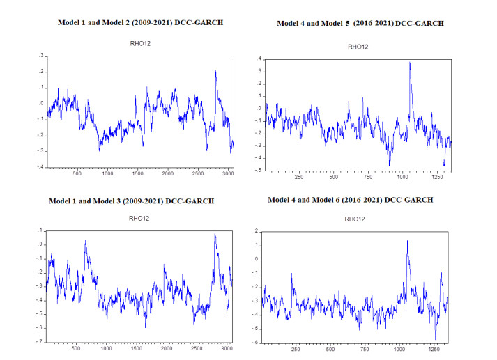
In this study, we examine the nexus between crude oil prices, clean energy investments, technology companies, and energy democracy. Our dataset incorporates four variables which are S & P Global Clean Energy Index (SPClean), Brent crude oil futures (Brent), CBOE Volatility Index (VIX), and NASDAQ 100 Technology Sector (DXNT) daily prices between 2009 and 2021. The novelty of our study is that we included technology development and market fear as important factors and assess their impact on clean energy investments. DCC-GARCH models are utilized to analyze the spillover impact of market fear, oil prices, and technology company stock returns to clean energy investments. According to our findings when oil prices decrease, the volatility index usually responds by increasing which means that the market is afraid of oil price surges. Renewable investments also tend to decrease in that period following the oil price trend. Moreover, a positive relationship between technology stocks and renewable energy stock returns also exists.

References

[1]	Adams S, Acheampong A (2019) Reducing Carbon Emissions: The Role of Renewable Energy and Democracy. J Clean Prod 240: 118245.
[2]	Alhassan S, Alade SA (2017) Income and Democracy in Sub-Sahara Africa. J Econ Sust Dev 8: 67-73.
[3]	Alola AA, Bekun VF, Sarkodie AS (2019) Dynamic impact of trade policy, economic growth, fertility rate, renewable and non-renewable energy consumption on ecological footprint in Europe. Sci Total Environ 685: 702-709. doi: 10.1016/j.scitotenv.2019.05.139
[4]	Barrett S, Graddy K (2000) Freedom, growth, and the environment. Environ Dev Econ 5: 433-456. doi: 10.1017/S1355770X00000267
[5]	Becker S, Kunze C (2014) Transcending community energy: collective and politically motivated projects in renewable energy (CPE) across Europe. People Place Policy 8: 180-191.
[6]	Bollerslev T (1986) Generalized Autoregressive Conditional Heteroscedasticity. J Econometrics 31: 307-327. doi: 10.1016/0304-4076(86)90063-1
[7]	Bondia R, Ghosh S, Kanjilal K (2016) International Crude Oil Prices and the Stock Prices of Clean Energy and Technology Companies: Evidence from Non-linear Cointegration Tests with Unknown Structural Breaks. Energy 101: 558-565. doi: 10.1016/j.energy.2016.02.031
[8]	Burke M, Stephens CJ (2018) Political power and renewable energy futures: A critical review. Energy Res Social Sci 35: 78-93. doi: 10.1016/j.erss.2017.10.018
[9]	Corbet S, Goodell WJ, Günay S (2020) Co-movements and spillovers of oil and renewable firms under extreme conditions: new evidence from negative WTI prices during COVID-19. Energy Econ 92: 104978.
[10]	Diebold FX, Yilmaz K (2012) Better to Give than to Receive: Predictive Directional Measurement of Volatility Spillovers. Int J Forecasting 28: 57-66. doi: 10.1016/j.ijforecast.2011.02.006
[11]	Dutta A (2017) Oil Price Uncertainty and Clean Energy Stock Returns: New Evidence from Crude Oil Volatility Index. J Clean Prod 164: 1157-1166. doi: 10.1016/j.jclepro.2017.07.050
[12]	Engle R (1982) Autoregressive Conditional Heteroscedasticity with Estimates of the Variance of United Kingdom Inflation. Econometrica 50: 987-1007. doi: 10.2307/1912773
[13]	Engle R, Ng KV (1993) Measuring and Testing the Impact of News on Volatility. J Financ 48: 1749-1778. doi: 10.1111/j.1540-6261.1993.tb05127.x
[14]	Farzin YH, Bond CA (2006) Democracy and Environmental Quality. J Dev Econ 81: 213-235. doi: 10.1016/j.jdeveco.2005.04.003
[15]	Ferrer R, Shahzad SJH, López R, et al. (2018) Time and Frequency Dynamics of Connectedness Between Renewable Energy Stocks and Crude Oil Prices. Energy Econ 76: 1-20. doi: 10.1016/j.eneco.2018.09.022
[16]	Inchauspe J, Ripple RD, Trück S (2015) The Dynamics of Returns on Renewable Energy Companies: A State-Space Approach. Energy Econ 48: 325-335. doi: 10.1016/j.eneco.2014.11.013
[17]	Kumar S, Managi S, Matsuda A (2012) Stock Prices of Clean Energy Firms, Oil and Carbon Markets: A Vector Autoregressive Analysis. Energy Econ 34: 215-226. doi: 10.1016/j.eneco.2011.03.002
[18]	Lv Z (2017) The effect of democracy on CO₂ emissions in emerging countries: Does the level of income matter? Renew Sust Energy Rev 72: 900-906.
[19]	Maji IK (2015) Does Clean Energy Contribute to Economic Growth? Evidence from Nigeria. Energy Rep 1: 145-150. doi: 10.1016/j.egyr.2015.06.001
[20]	Nguyen C, Schinckus C, Thanh SD (2019) Economic Integration and CO₂ Emissions: Evidence from Emerging Economies. Climate Dev 12: 369-384. doi: 10.1080/17565529.2019.1630350
[21]	Nguyen C, Schinckus C, Thanh SD (2018) The ambivalent role of institutions in the CO₂ Emissions: The case of Emerging Countries. Int J Energy Econ Policy 8: 7-17.
[22]	Nguyen C, Schinckus C, Dinh TS, Bensemann J, et al. (2019) Global Emissions: A New Contribution from the Shadow Economy. Int J Energy Econ Policy 9: 320-337.
[23]	Nguyen C, Ha-Le T, Schinckus C, et al. (2020) Determinants of agricultural emissions: panel data evidence from a global sample. Environ Dev Econ 26: 109-130. doi: 10.1017/S1355770X20000315
[24]	Omri A, Mabrouk NB, Sassi-Tmar A (2015) Modeling the Causal Linkages Between Nuclear Energy, Renewable Energy and Economic Growth in Developed and Developing Countries. Working Papers 2015-623, Department of Research, Ipag Business School.
[25]	Reboredo JC (2015) Is There Dependence and Systemic Risk Between Oil and Renewable Energy Stock Prices? Energy Econ 48: 32-45.
[26]	Roberts JT, Parks BC (2007) Fueling Injustice: Globalization, Ecologically Unequal Exchange and Climate Change. Globalizations 4: 193-210.
[27]	Sadorsky P (2012) Correlations and Volatility Spillovers Between Oil Prices and the Stock Prices of Clean Energy and Technology Companies. Energy Econ 34: 248-255. doi: 10.1016/j.eneco.2011.03.006
[28]	Symitsi E, Chalvatzis KJ (2019) The economic value of Bitcoin: A portfolio analysis of currencies, gold, oil and stocks. Res Int Bus Financ 48: 97-110. doi: 10.1016/j.ribaf.2018.12.001
[29]	Szulecki K, Overland I (2018) Energy democracy as a process, an outcome a goal: A conceptual review. Energy Res Social Sci 69: 101768.
[30]	Torras M, Boyce KJ (1998) Income, inequality, and pollution: a reassessment of the environmental Kuznets Curve. Ecol Econ 25: 147-160. doi: 10.1016/S0921-8009(97)00177-8
[31]	Ulusoy V, Özdurak C (2018) The Impact of Oil Price Volatility to Oil and Gas Company Stock Returns and Emerging Economies. Int J Energy Econ Policy Econ J 8: 144-158.
[32]	Usman O, Iortile IB, Ike NG (2020) Enhancing sustainable electricity consumption in a large ecological reserve-based country: the role of democracy, ecological footprint, economic growth, and globalisation in Brazil. Environ Sci Pollut Res 27: 13370-13383. doi: 10.1007/s11356-020-07815-3
[33]	Usman O, Olanipekun OI, Iorember TP, et al. (2020) Modelling environmental degradation in South Africa: the effects of energy consumption, democracy, and globalization using innovation accounting tests. Environ Sci Pollut Res 27: 8334-8349. doi: 10.1007/s11356-019-06687-6

Reader Comments

Your name:*

Email:*
© 2021 the Author(s), licensee AIMS Press. This is an open access article distributed under the terms of the Creative Commons Attribution License (http://creativecommons.org/licenses/by/4.0)