How can carbon markets drive the development of renewable energy sector? Empirical evidence from China

Jiamin Cheng; Yuanying Jiang; Jiamin Cheng; Yuanying Jiang

doi:10.3934/DSFE.2024010

Data Science in Finance and Economics

2024, Volume 4, Issue 2: 249-269. doi: 10.3934/DSFE.2024010

Previous Article Next Article

Research article

How can carbon markets drive the development of renewable energy sector? Empirical evidence from China

Jiamin Cheng ¹,
Yuanying Jiang ^{1,2
,
,}

1.
School of Mathematics and Statistics, Guilin University of Technology, Guilin, 541004, China
2.
Guangxi Colleges and Universities Key Laboratory of Applied Statistics, Guilin, 541004, China

Received: 06 March 2024 Revised: 22 March 2024 Accepted: 10 April 2024 Published: 08 May 2024
JEL Codes: C1, C12, C15, C16, G1, G18

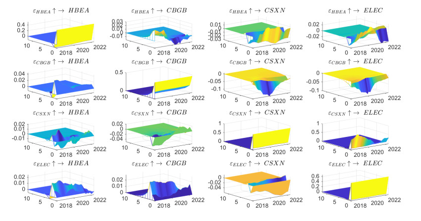
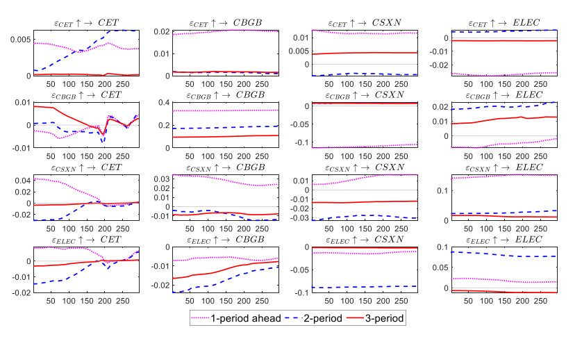
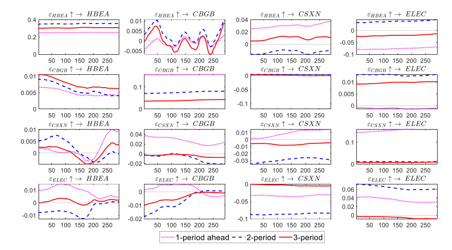
The reduction of carbon emissions has attracted significant global attention. This paper empirically analyzes the dynamic nonlinear linkages among carbon markets, green bonds, clean energy, and electricity markets by constructing DCC-GARCH and TVP-VAR-SV models, and places the four markets under a unified framework to analyze the volatility risk from a time-varying perspective, thereby enriching the research on China's carbon market and renewable energy sector. We found that extreme events have a significant impact on the dynamic connectivity among the four markets. The analysis of the shock impact indicates that the carbon market has a positive effect on the power market in the short and medium terms, but has a mitigating impact in the long term. Especially, when the other markets are hit, the carbon market has evident fluctuation in 2020. The green bond market has a positive influence on the carbon market, whereas the power market demonstrates adverse effects in the short and medium terms. The New Energy Index negatively impacts the power market in the short and medium terms, but is expected to have a positive effect after 2020, highlighting the growing need for renewable energy in the power system transformation. According to the findings mentioned above, we put forward appropriate recommendations.
- carbon market,
- green bonds,
- clean energy,
- electricity market,
- TVP-VAR-SV
Citation: Jiamin Cheng, Yuanying Jiang. How can carbon markets drive the development of renewable energy sector? Empirical evidence from China[J]. Data Science in Finance and Economics, 2024, 4(2): 249-269. doi: 10.3934/DSFE.2024010

Related Papers:

Abstract

The reduction of carbon emissions has attracted significant global attention. This paper empirically analyzes the dynamic nonlinear linkages among carbon markets, green bonds, clean energy, and electricity markets by constructing DCC-GARCH and TVP-VAR-SV models, and places the four markets under a unified framework to analyze the volatility risk from a time-varying perspective, thereby enriching the research on China's carbon market and renewable energy sector. We found that extreme events have a significant impact on the dynamic connectivity among the four markets. The analysis of the shock impact indicates that the carbon market has a positive effect on the power market in the short and medium terms, but has a mitigating impact in the long term. Especially, when the other markets are hit, the carbon market has evident fluctuation in 2020. The green bond market has a positive influence on the carbon market, whereas the power market demonstrates adverse effects in the short and medium terms. The New Energy Index negatively impacts the power market in the short and medium terms, but is expected to have a positive effect after 2020, highlighting the growing need for renewable energy in the power system transformation. According to the findings mentioned above, we put forward appropriate recommendations.

References

[1]	Arif M, Naeem MA, Farid S, et al. (2021) Diversifier or more? Hedge and safe haven properties of green bonds during COVID-19. Energ Policy 168: 113102. https://doi.org/10.1016/j.enpol.2022.113102 doi: 10.1016/j.enpol.2022.113102
[2]	Avkiran NK, Cai L (2014) Identifying distress among banks prior to a major crisis using non-oriented super-SBM. Ann Oper Res 217: 31–53. https://doi.org/10.1007/s10479-014-1568-8 doi: 10.1007/s10479-014-1568-8
[3]	Broock WA, Scheinkman JA, Dechert WD, et al. (1996) A test for independence based on the correlation dimension. Economet Rev 15: 197–235. https://doi.org/10.1080/07474939608800353 doi: 10.1080/07474939608800353
[4]	Bloomberg NEF (2020) Power sector to spend $5 billion on software by 2025.
[5]	Chang K, Ge F, Zhang C, et al. (2018) The dynamic linkage effect between energy and emissions allowances price for regional emissions trading scheme pilots in China. Renew Sust Energy Rev 98: 415–425. https://doi.org/10.1016/j.rser.2018.09.023 doi: 10.1016/j.rser.2018.09.023
[6]	Chai S, Chu W, Zhang Z, et al. (2022) Dynamic nonlinear connectedness between the green bonds, clean energy, and stock price: the impact of the COVID-19 pandemic. Ann Oper Res 2022: 1–28. https://doi.org/10.1007/s10479-021-04452-y doi: 10.1007/s10479-021-04452-y
[7]	Chan HY, Merdekawati M, Suryadi B (2022) Bank climate actions and their implications for the coal power sector. Energy Strateg Rev 39: 100799. https://doi.org/10.1016/j.esr.2021.100799 doi: 10.1016/j.esr.2021.100799
[8]	Chen Y, Jiang Y (2023) Integration of green energy equity and fossil energy markets in different time scales: evidence from the US, Europe and China. Int J Environ Pollut 72: 198–221. https://doi.org/10.1504/IJEP.2023.10060227 doi: 10.1504/IJEP.2023.10060227
[9]	Esmaeili P, Rafei M (2021) Dynamics analysis of factors affecting electricity consumption fluctuations based on economic conditions: Application of SVAR and TVP-VAR models. Energy 226: 120340. https://doi.org/10.1016/j.energy.2021.120340 doi: 10.1016/j.energy.2021.120340
[10]	Engle Ⅲ RF, Sheppard K (2001) Theoretical and empirical properties of dynamic conditional correlation multivariate GARCH. https://doi.org/10.3386/w8554
[11]	Engle RF (2002) A simple class of multivariate generalized autoregressive conditional heteroskedasticity models. J Bus Econ Stat 20: 339–350.
[12]	Gong X, Shi R, Xu J, et al. (2021) Analyzing spillover effects between carbon and fossil energy markets from a time-varying perspective. Appl Energ 285: 116384. https://doi.org/10.1016/j.apenergy.2020.116384 doi: 10.1016/j.apenergy.2020.116384
[13]	Hanif W, Hernandez JA, Mensi W, et al. (2021) Nonlinear dependence and connectedness between clean renewable energy sector equity and European emission allowance prices. Energ Econ 101: 105409. https://doi.org/10.1016/j.eneco.2021.105409 doi: 10.1016/j.eneco.2021.105409
[14]	He L, Zhang L, Zhong Z, et al. (2019) Green credit, renewable energy investment and green economy development: Empirical analysis based on 150 listed companies of China. J Clean Prod 208: 363–372. https://doi.org/10.1016/j.jclepro.2018.10.119 doi: 10.1016/j.jclepro.2018.10.119
[15]	He Z (2020) Dynamic impacts of crude oil price on Chinese investor sentiment: Nonlinear causality and time-varying effect. Int Rev Econ Financ 66: 131–153. https://doi.org/10.1016/j.irej.iref.2019.11.004 doi: 10.1016/j.irej.iref.2019.11.004
[16]	Hammoudeh S, Ajmi AN, Mokni K (2021) Relationship between green bonds and financial and environmental variables: A novel time-varying causality. Energ Econ 92: 104941. https://doi.org/10.1016/j.eneco.2020.104941 doi: 10.1016/j.eneco.2020.104941
[17]	Li H, Li J, Jiang Y (2023) Exploring the Dynamic Impact between the Industries in China: New Perspective Based on Pattern Causality and Time-Varying Effect. Systems 11: 318. https://doi.org/10.3390/systems11070318 doi: 10.3390/systems11070318
[18]	IRENA (2019) Innovation landscape for a renewable-powered future: Solutions to integrate variable renewables. Int Renew Energ Agency, Abu Dhabi.
[19]	Ji Q, Zhang D, Geng J (2018) Information linkage, dynamic spillovers in prices and volatility between the carbon energy markets. J Clean Prod 198: 972–978. https://doi.org/10.1016/j.jclepro.2018.07.126 doi: 10.1016/j.jclepro.2018.07.126
[20]	Ji Q, Xia T, Liu F, et al (2019) The information spillover between carbon price and power Sector returns: Evidence from the major European electricity companies. J Clean Prod 208: 1178–1187. https://doi.org/10.1016/j.jclepro.2018.10.167 doi: 10.1016/j.jclepro.2018.10.167
[21]	Li P, Zhang H, Yuan Y, et al. (2021) Time-varying impacts of carbon price drives in the EU ETS: A TETS: A TVP-VAR Analysis. Front Env Sci 9: 651791. https://doi.org/10.3389/fenvs.2021.651791 doi: 10.3389/fenvs.2021.651791
[22]	Li Y, Nie D, Li B, et al. (2020) The Spillover Effect between Carbon Emission Trading Price and Power Company Stock Price in China. Sustainability 12: 6573. https://doi.org/10.3390/su12166573 doi: 10.3390/su12166573
[23]	Li F, Cao X, Ou R (2021) A network-based evolutionary analysis of the diffusion of cleaner energy substitution in enterprises: the roles of PEST factors. Energ Policy 156: 112385. https://doi.org/10.1016/j.enpol.2021.112385 doi: 10.1016/j.enpol.2021.112385
[24]	Lin Z, Liao X, Jia H (2023) Could green finance facilitate low-carbon transformation of power generation? Some evidence from China. Int J Clim Chang Strategies Manage 15: 141–158. https://doi.org/10.1108/IJCCSM-03-2022-0039 doi: 10.1108/IJCCSM-03-2022-0039
[25]	Nong H, Guan Y, Jiang Y (2022) Identifying the volatility spillover risks between crude oil price and China's clean energy market. Electro Res Arch 30: 4593–4618. https://doi.org/10.3934/era.2022233 doi: 10.3934/era.2022233
[26]	Nguyen TTH, Naeem MA, Balli F, et al. (2021) Time-frequency co-movement among green bonds, stocks, commodities, clean energy, and conventional bonds. Financ Res Lett 40: 101739. https://doi.org/10.1016/j.frl.2020.101739 doi: 10.1016/j.frl.2020.101739
[27]	Nakajima J (2011) Time-varying Parameter VAR Model with Stochastic Volatility: An Overview of Methodology and Empirical Applications. Inst Monetary Econ Stud, Bank of Japan.
[28]	Pham L (2021) Frequency connectedness and cross-quantile dependence between green bond and green equity markets. Energ Econ 98: 105257. https://doi.org/10.1016/j.eneco.2021.105257 doi: 10.1016/j.eneco.2021.105257
[29]	Piotr F, Witold O (2018) Nonlinear granger causality between grains and livestock. Agr Econ 64: 328–336. https://doi.org/10.17221/376/2016-AGRICECON doi: 10.17221/376/2016-AGRICECON
[30]	Primiceri GE (2005) Time-Varying Structural Vector Autoregressions and Monetary Policy. Rev Econ Stud 72: 821–852.
[31]	Ren X, Cheng C, Wang Z, et al. (2021) Spillover and dynamic effects of energy transition and economic growth on carbon dioxide emissions for the European Union: a dynamic spatial panel model. Sustain Devt 29: 228–242. https://doi.org/10.1002/sd.2144 doi: 10.1002/sd.2144
[32]	Ren X, Li Y, Wen F, et al. (2022) The interrelationship between the carbon market and the green bonds market: Evidence from wavelet quantile-on-quantile method. Technol Forecast Soc Chang 179: 121611. https://doi.org/10.1016/j.techfore.2022.121611 doi: 10.1016/j.techfore.2022.121611
[33]	Reboredo JC, Ugolini A (2020) Price connectedness between green bond and financial markets. Econ Model 88: 25–38. https://doi.org/10.1016/j.econmod.2019.09.004 doi: 10.1016/j.econmod.2019.09.004
[34]	Samuel Asante Gyamerah, Clement Asare (2024) A critical review of the impact of uncertainties on green bonds. Green Financ 6: 78–91. https://doi: 10.3934/GF.2024004 doi: 10.3934/GF.2024004
[35]	Strantzali E, Aravossis K (2016) Decision making in renewable energy investments: A review. Renew Sust Energ Rev 55: 885–898. https://doi.org/10.1016/j.rser.2015.11.021 doi: 10.1016/j.rser.2015.11.021
[36]	Wen F, Zhao H, Zhao L, et al. (2022) What drive carbon price dynamics in China. Int Rev Financ Anal 79: 101999. https://doi.org/10.1016/j.irfa.2021.101999 doi: 10.1016/j.irfa.2021.101999
[37]	Wu Y, Wang J, Ji S, et al. (2020) Renewable energy investment risk assessment for nations along China's Belt & Road Initiative: An ANP-cloud model method. Energy 190: 116381. https://doi.org/10.1016/j.energy.2019.116381 doi: 10.1016/j.energy.2019.116381
[38]	Xiao H, Zhang Z, Wang A, et al. (2021) Evaluating energy security in China: a subnational analysis. In China's Energy Security: Analysis, Assessment and Improvement, 119–137. https://doi.org/10.1142/97817863492240005
[39]	Yang L (2022) Idiosyncratic information spillover and connectedness network between the electricity and carbon markets in Europe. J Commod Mark 25: 100185. https://doi.org/10.1016/j.jcomm.2021.100185 doi: 10.1016/j.jcomm.2021.100185
[40]	Yin G, Li B, Fedorova N, et al. (2021) Orderly retire China's coal-fired power capacity via capacity payments to support renewable energy expansion. Iscience 24. https://doi.org/10.1016/j.isci.2021.103287 doi: 10.1016/j.isci.2021.103287
[41]	Zhao L, Liu W, Zhou M, et al. (2022) Extreme event shocks and dynamic volatility interactions: The stock, commodity, and carbon markets in China. Financ Res Lett 47: 102645.https://doi.org/10.1016/j.frl.2021.102645 doi: 10.1016/j.frl.2021.102645
[42]	Zhao X, Li Q, Xue W, et al. (2022) Research on ultra-short-term load forecasting based on real-time electricity price and window-based XGBoost model. Energies 15: 7367. https://doi.org/10.3390/en15197367 doi: 10.3390/en15197367
[43]	Zhao Y, Zhou Z, Zhang K, et al. (2023) Research on spillover effect between carbon market and electricity market: Evidence from Northern Europe. Energy 263: 126107. https://doi.org/10.1016/j.energy.2022.126107 doi: 10.1016/j.energy.2022.126107
[44]	Zhou K, Li Y (2019) Influencing factors and fluctuation characteristics of China's carbon emission trading price. Physica A 524: 459–474. https://doi.org/10.1016/j.physa.2019.04.249 doi: 10.1016/j.physa.2019.04.249
[45]	Zhou D, Chen B, Li J, et al. (2021) China's economic growth, energy efficiency, and industrial development: Nonlinear effects on carbon dioxide emissions. Discrete Dyn Nat Soc 2021: 1–17. https://doi.org/10.1155/2021/5547092 doi: 10.1155/2021/5547092
[46]	Zhou Y, Wu S, Liu Z, et al. (2023) The asymmetric effects of climate risk on higher-moment connectedness among carbon, energy and metals markets. Nat Commun 14: 7157. https://doi.org/10.1038/s41467-023-42925-9 doi: 10.1038/s41467-023-42925-9

Reader Comments

Your name:*

Email:*
© 2024 the Author(s), licensee AIMS Press. This is an open access article distributed under the terms of the Creative Commons Attribution License (http://creativecommons.org/licenses/by/4.0)