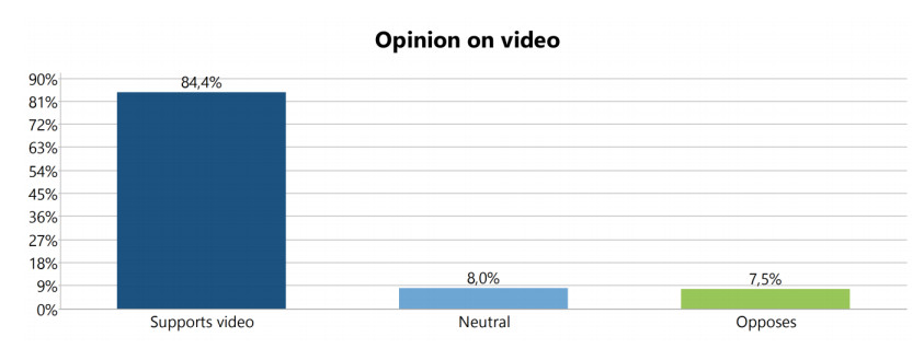
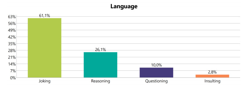
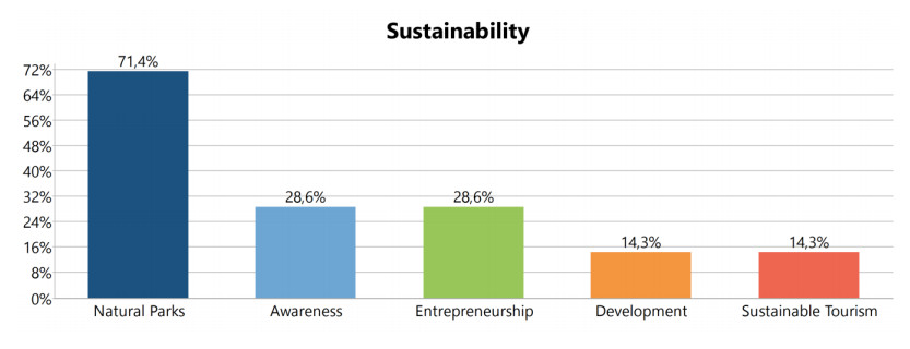
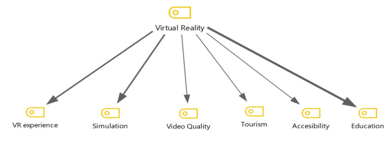
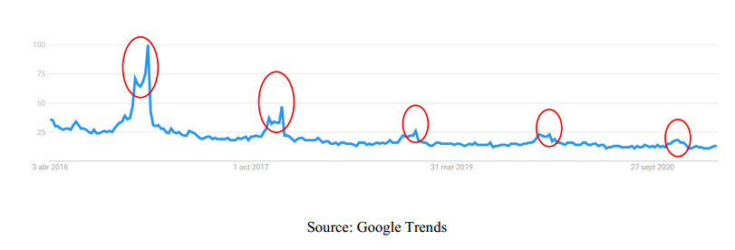
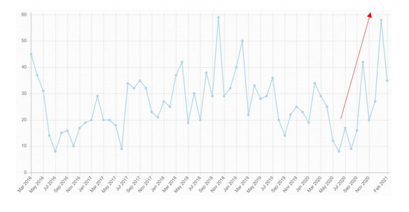
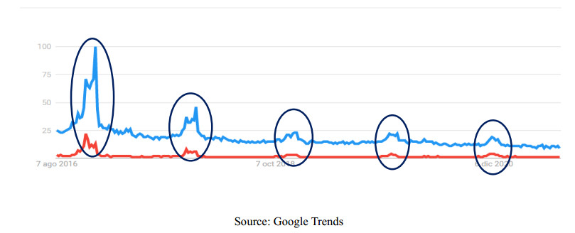
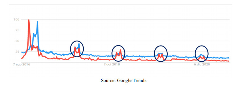
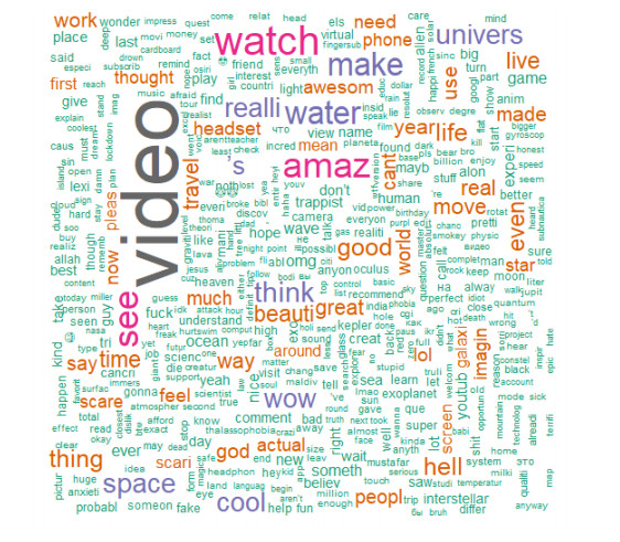
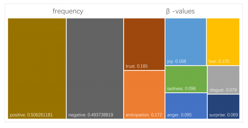
The purpose of this research is to highlight the importance of periodically analyzing the data obtained from the technological sources used by customers, such as user comments on social networks and videos, using qualitative data analysis software. This research analyzes user sentiments, words, and opinions about virtual reality (VR) videos on YouTube in order to explore user reactions to such videos, as well as to establish whether this technology contributes to the sustainability of natural environments. User-generated data can provide important information for decision making about future policies of companies that produce video content. The results of our analysis of 12 videos revealed that users predominantly perceived these videos positively. This conclusion was supported by the findings of an opinion and text analysis, which identified positive reviews for videos and channels with many followers and large numbers of visits. The features such as the quality of the video and the accessibility of technology were appreciated by the viewers, whereas videos that are 100% VR and require special glasses to view them do not have as many visits. However, VR was seen to be a product which viewers were interested in and, according to Google, there are an increasing number of searches and sales of VR glasses in holiday seasons. Emotions of wonder and joy are more evident than emotions of anger or frustration, so positive feelings can be seen to be predominant.
Citation: Pedro R. Palos Sánchez, José A. Folgado-Fernández, Mario Alberto Rojas Sánchez. Virtual Reality Technology: Analysis based on text and opinion mining[J]. Mathematical Biosciences and Engineering, 2022, 19(8): 7856-7885. doi: 10.3934/mbe.2022367
The purpose of this research is to highlight the importance of periodically analyzing the data obtained from the technological sources used by customers, such as user comments on social networks and videos, using qualitative data analysis software. This research analyzes user sentiments, words, and opinions about virtual reality (VR) videos on YouTube in order to explore user reactions to such videos, as well as to establish whether this technology contributes to the sustainability of natural environments. User-generated data can provide important information for decision making about future policies of companies that produce video content. The results of our analysis of 12 videos revealed that users predominantly perceived these videos positively. This conclusion was supported by the findings of an opinion and text analysis, which identified positive reviews for videos and channels with many followers and large numbers of visits. The features such as the quality of the video and the accessibility of technology were appreciated by the viewers, whereas videos that are 100% VR and require special glasses to view them do not have as many visits. However, VR was seen to be a product which viewers were interested in and, according to Google, there are an increasing number of searches and sales of VR glasses in holiday seasons. Emotions of wonder and joy are more evident than emotions of anger or frustration, so positive feelings can be seen to be predominant.

| [1] |
A. Porreca, F. Scozzari, M. Di Nicola, Using text mining and sentiment analysis to analyze YouTube Italian videos concerning vaccination, BMC Public Health, 20 (2020), 1–9. https://doi.org/10.1186/s12889-020-8342-4 doi: 10.1186/s12889-020-8342-4

|
| [2] |
Z. Li, R. Li, G. Jin, Sentiment analysis of danmaku videos based on Naïve Bayes and sentiment dictionary, IEEE Access, 8 (2020), 75073–75084. https://doi.org/10.1109/ACCESS.2020.2986582 doi: 10.1109/ACCESS.2020.2986582
|
| [3] |
G. S. Chauhan, Y. K. Meena, YouTube video ranking by aspect-based sentiment analysis on user feedback, Soft Comput. Signal Process., (2019), 63–71. https://doi.org/10.1007/978-981-13-3600-3_6 doi: 10.1007/978-981-13-3600-3_6
|
| [4] |
T. Tomihira, A. Otsuka, A. Yamashita A, T. Satoh, Multilingual emoji prediction using BERT for sentiment analysis, Int. J. Web Inf. Syst., 16 (2020), 265–280. https://doi.org/10.1108/IJWIS-09-2019-0042 doi: 10.1108/IJWIS-09-2019-0042
|
| [5] | R. Botsman, R. Rogers, What's mine is yours, The rise of collaborative consumption. New York: HarperCollins, (2010). |
| [6] |
S. M. C. Loureiro, J. Guerreiro, F. Ali, 20 years of research on virtual reality and augmented reality in tourism context: A text-mining approach, Tour. Manag., 77 (2020), 104028. https://doi.org/10.1016/j.tourman.2019.104028 doi: 10.1016/j.tourman.2019.104028
|
| [7] |
R. G. Bilro, S. M. C. Loureiro, J. Guerreiro, Exploring online customer engagement with hospitality products and its relationship with involvement, emotional states, experience and brand advocacy, J. Hosp. Market. Manag., 28 (2019), 147–171. https://doi.org/10.1080/19368623.2018.1506375 doi: 10.1080/19368623.2018.1506375
|
| [8] |
S. M. C. Loureiro, J. Guerreiro, S. Eloy, D. Langaro, P. Panchapakesan, Understanding the use of Virtual Reality in Marketing: A text mining-based review, J. Bus. Res., 100 (2019), 514–530. https://doi.org/10.1016/j.jbusres.2018.10.055 doi: 10.1016/j.jbusres.2018.10.055
|
| [9] |
M. Wedel, E. Bigné, J. Zhang, Virtual and augmented reality: Advancing research in consumer marketing, Int. J. Res. Mark., 37 (2020), 443–465. https://doi.org/10.1016/j.ijresmar.2020.04.004 doi: 10.1016/j.ijresmar.2020.04.004
|
| [10] |
F. Velicia-Martin, J. A. Folgado-Fernández, P. R. Palos-Sánchez, B. López-Catalán, mWOM Business Strategies: Factors Affecting Recommendations, J. Comput. Inf. Syst., (2022), 1–14. https://doi.org/10.1080/08874417.2022.2041504 doi: 10.1080/08874417.2022.2041504
|
| [11] |
S. Moro, P. Rita, P. Ramos, J. Esmeraldo, Analysing recent augmented and virtual reality developments in tourism, J. Hosp. Tour. Technol., 10 (2019), 571–586. https://doi.org/10.1108/JHTT-07-2018-0059 doi: 10.1108/JHTT-07-2018-0059
|
| [12] |
S. M. C. Loureiro, H. Roschk H, Differential effects of atmospheric cues on emotions and loyalty intention with respect to age under online/offline environment, J. Retail. Consum. Serv., 21 (2014), 211–219. https://doi.org/10.1016/j.jretconser.2013.09.001 doi: 10.1016/j.jretconser.2013.09.001
|
| [13] |
X. Xu, Y. Li, The antecedents of customer satisfaction and dissatisfaction toward various types of hotels: A text mining approach, Int. J. Hosp. Manag., 55 (2016), 57–69. https://doi.org/10.1016/j.ijhm.2016.03.003 doi: 10.1016/j.ijhm.2016.03.003
|
| [14] |
L. Serrano, A. Ariza-Montes, M. Nader, A. Sianes, R. Law, Exploring preferences and sustainable attitudes of Airbnb green users in the review comments and ratings: A text mining approach, J. Sustain. Tour., 28 (2020), 1–19. https://doi.org/10.1080/09669582.2020.1838529 doi: 10.1080/09669582.2020.1838529
|
| [15] |
X. Wu, Q., Zhi, Impact of shared economy on urban sustainability: From the perspective of social, economic, and environmental sustainability, Energy Proced., 104 (2016), 191–196. https://doi.org/10.1016/j.egypro.2016.12.033 doi: 10.1016/j.egypro.2016.12.033
|
| [16] |
H. Han, B. Meng, W. Kim, Emerging bicycle tourism and the theory of planned behavior, J. Sustain. Tour., 25 (2017), 292–309. https://doi.org/10.1080/09669582.2016.1202955 doi: 10.1080/09669582.2016.1202955
|
| [17] | C. Midgett, J. S. Bendickson, J. Muldoon, S. J. Solomon, The sharing economy and sustainability: A case for Airbnb, Small Bus. Inst. J., 13 (2018), 51–71. |
| [18] | A. N. Srivastava, M. Sahami, Text mining: Classification, clustering, and applications, New York, NY, Chapman & Hall/CRC, (2009). |
| [19] |
C. Koltinger, A. Dickinger, Analyzing destination branding and image from online sources: A web content mining approach, J. Bus. Res. 68 (2015), 1836–1843. https://doi.org/10.1016/j.jbusres.2015.01.011 doi: 10.1016/j.jbusres.2015.01.011
|
| [20] | S. M. C. Loureiro, J. Guerreiro, F. Ali, 20 years of research on virtual reality and augmented reality in tourism context: A text-mining approach, Tour. Manag., 77 (2020), 104028. |
| [21] |
S. Rangelova, E. Andre, A survey on simulation sickness in driving applications with Virtual Reality Head-mounted displays, Presence V. Augmented R., 27 (2019), 15–31. https://doi.org/10.1162/pres_a_00318 doi: 10.1162/pres_a_00318
|
| [22] |
J. Martínez-Navarro, E. Bigné, J. Guixeres, M. Alcaniz, C. Torrecilla, The influence of virtual reality in e-commerce, J. Bus. Res., 100 (2019), 475–482. https://doi.org/10.1016/j.jbusres.2018.10.054 doi: 10.1016/j.jbusres.2018.10.054
|
| [23] | K. Zhang, J. Suo, J. Chen, X. Liu, L. Gao, Design and implementation of fire safety education system on campus based on virtual reality technology, Federated Conference on Computer Science and Information Systems (FedCSIS), (2017), 1297–1300. |
| [24] | C. Anthes, R. J. García-Hernández, M. Wiedemann, D. Kranzlmüller, State of the art of virtual reality technology, IEEE Aerospace Conference, (2016), 1–19. |
| [25] |
C. Flavián, S. Ibáñez-Sánchez, C. Orús, Integrating virtual reality devices into the body: effects of technological embodiment on customer engagement and behavioral intentions toward the destination, J. Travel Tour. Mark., 36 (2019), 847–863. https://doi.org/10.1080/10548408.2019.1618781 doi: 10.1080/10548408.2019.1618781
|
| [26] | M. A. Gigante, Virtual Reality: Definitions, History and Applications, in Virtual Reality Systems (eds. R. A. Earnshaw, M. A. Gigante and H. Jones), Boston, Academic Press, (1993), 3–14. |
| [27] | P. Disztinger, S. Schlögl, A. Groth, Technology Acceptance of Virtual Reality for Travel Planning, in Information and Communication Technologies in Tourism 2017 (Eds. R. Schegg and B. Stangl), Cham, Springer International Publishing, (2017), 255–268. |
| [28] |
I. P. Tussyadiah, D. Wang, T. H. Jung, M. C. Tom Dieck, Virtual reality, presence, and attitude change: Empirical evidence from tourism, Tourism Manage, 66 (2018), 140–154. https://doi.org/10.1016/j.tourman.2017.12.003 doi: 10.1016/j.tourman.2017.12.003
|
| [29] |
M. Fagan, C. Kilmon, V. Pandey, Exploring the adoption of a virtual reality simulation: The role of perceived ease of use, perceived usefulness and personal innovativeness, Campus-Wide Inf. Sys., 29 (2012), 117–127. https://doi.org/10.1108/10650741211212368 doi: 10.1108/10650741211212368
|
| [30] | M. Mihelj, D. Novak, S. Beguš, Virtual Reality Technology and Applications, Dordrecht, Springer Netherlands, (2014). |
| [31] |
Y. C. Huang, K. F. Backman, S. J. Backman, L. L. Chang, Exploring the implications of Virtual Reality Technology in tourism marketing: An integrated research framework, Int. J. Tour. Res., 18 (2016), 116–128. https://doi.org/10.1002/jtr.2038 doi: 10.1002/jtr.2038
|
| [32] |
D. M. Tamás, Introduction to the WIPO Pearl patent terminology database, Fordítástudomány, 23 (2021), 49–62. https://doi.org/10.35924/fordtud.23.1.3 doi: 10.35924/fordtud.23.1.3
|
| [33] |
D. Babčanová, J. Šujanová, D. Cagáňová, N. Horňáková, H. Hrablik Chovanová, Qualitative and quantitative analysis of social network data intended for brand management, Wirel. Netw., 27 (2019), 1–8. https://doi.org/10.1007/s11276-019-02052-0 doi: 10.1007/s11276-019-02052-0
|
| [34] |
Z. T. Osakwe, I. Ikhapoh, B. K. Arora, O. M. Bubu, Identifying public concerns and reactions during the COVID-19 pandemic on Twitter: A text-mining analysis. Public Health Nur., 38 (2021), 145–151. https://doi.org/10.1111/phn.12843 doi: 10.1111/phn.12843
|
| [35] |
A. Brait, Attitudes of Austrian history teachers towards memorial site visits, Eine Analyse mithilfe von MAXQDA zeitgeschichte, 47 (2020), 441–466. https://doi.org/10.14220/zsch.2020.47.4.441 doi: 10.14220/zsch.2020.47.4.441
|
| [36] |
P. Kowalczuk, Consumer acceptance of smart speakers: a mixed methods approach, J. Res. Interact. Mark., 12 (2018), 418–431. https://doi.org/10.1108/JRIM-01-2018-0022 doi: 10.1108/JRIM-01-2018-0022
|
| [37] |
R. P. S. Kaurav, K. Suresh, S. Narula, R. Baber, The new education policy 2020 using Twitter mining, J. Content Community Commun., 12 (2021), 4–13. https://doi.org/10.31620/JCCC.12.20/02 doi: 10.31620/JCCC.12.20/02
|
| [38] | D. H. Choi, A. Dailey-Hebert, J. Simmons Estes, Emerging Tools and Applications of Virtual Reality in Education: IGI Global, (2016). |
| [39] |
M. A. Ríos-Martín, J. A. Folgado-Fernández, P. R. Palos-Sanchez, P. Castejón-Jiménez, The impact of the environmental quality of online feedback and satisfaction when exploring the critical factors for Luxury Hotels, Sustainability, 12 (2019), 299. https://doi.org/10.3390/su12010299 doi: 10.3390/su12010299
|
| [40] |
J. R. Saura, P. R. Palos-Sanchez, M. A. R. Martín, Attitudes expressed in online comments about environmental factors in the Tourism sector: An exploratory study, Int. J. Environ. Res. Public Health, 15 (2018), 553. https://doi.org/10.3390/ijerph15030553 doi: 10.3390/ijerph15030553
|
| [41] |
J. R. Saura, P. R. Palos-Sanchez, A. Grilo, Detecting indicators for startup business success: Sentiment analysis using text data mining, Sustainability, 11 (2019), 917. https://doi.org/10.3390/su11030917 doi: 10.3390/su11030917
|
| [42] |
J. R.Saura, A. Reyes-Menendez, P. Palos-Sanchez, Are Black Friday deals worth it? Mining Twitter users' sentiment and behavior response, J. Open Innov. Tech., Market Complex., 5 (2019), 58. https://doi.org/10.3390/joitmc5030058 doi: 10.3390/joitmc5030058
|
| [43] | J. R. Saura, A. Reyes-Menéndez, P. R. Palos-Sanchez, A Twitter sentiment analysis with machine learning: Identifying sentiment about #BlackFriday deals, Revista Espacios, 39 (2018). |
| [44] |
P. R. Palos-Sanchez, J. R.Saura, F. Debasa, The influence of social networks on the development of recruitment actions that favor user interface design and conversions in mobile applications powered by linked data, Mob. Inf. Syst., 2018 (2018). https://doi.org/10.1155/2018/5047017 doi: 10.1155/2018/5047017
|
| [45] |
P. R. Palos-Sanchez, J. R. Saura, M.B. Correia, Do tourism applications' quality and user experience influence its acceptance by tourists? Rev. Manag. Sci., 15 (2021), 1205–1241. https://doi.org/10.1007/s11846-020-00396-y doi: 10.1007/s11846-020-00396-y
|
| [46] |
D. Gefen, Reflections on the dimensions of trust and trustworthiness among online consumers, ACM SIGMIS Database: The Database for Advances in Information Systems, 33 (2002), 38–53. https://doi.org/10.1145/569905.569910 doi: 10.1145/569905.569910
|
| [47] |
A. C. Calheiros, S. Moro, P. Rita, Sentiment classification of consumer-generated online reviews using topic modeling, Hosp. Market. Manag., 26 (2017), 675–693. https://doi.org/10.1080/19368623.2017.1310075 doi: 10.1080/19368623.2017.1310075
|
| [48] |
S. Kang, S. Dove, H. Ebright, S. Morales, H. Kim, Does virtual reality affect behavioral intention? Testing engagement processes in a K-Pop video on YouTube, Comput. Hum. Behav. 123 (2021), 106875. https://doi.org/10.1016/j.chb.2021.106875 doi: 10.1016/j.chb.2021.106875
|
| [49] |
E. Filter, A Eckes, F. Fiebelkorn, A. G. Büssing, Virtual reality nature experiences involving wolves on YouTube: Presence, emotions, and attitudes in immersive and nonimmersive settings, Sustainability, 12 (2020), 3823. https://doi.org/10.3390/su12093823 doi: 10.3390/su12093823
|
| [50] |
C. C.W. Lim, J. Leung, J. Y.C. Chung, T. Sun, C. Gartner, J. Connor, et al., Content analysis of cannabis vaping videos on YouTube, Addiction, 116 (2021), 2443–2453. https://doi.org/10.1111/add.15424 doi: 10.1111/add.15424
|
| [51] |
J. Y. Lim, S. Kim, J. Kim, S. Lee, Identifying trends in nursing start-ups using text mining of YouTube content, Plos One, 15 (2020), e0226329. https://doi.org/10.1371/journal.pone.0226329 doi: 10.1371/journal.pone.0226329
|
| [52] |
N. Öztürk, S. Ayvaz, Sentiment analysis on Twitter: A text mining approach to the Syrian refugee crisis, Telemat. Inform., 35 (2018), 136–147. https://doi.org/10.1016/j.tele.2017.10.006 doi: 10.1016/j.tele.2017.10.006
|
| [53] |
A. Alarifi, M. Alsaleh, A. Al-Salman, Twitter turing test: Identifying social machines, Inf. Sci., 372 (2016), 332–346. https://doi.org/10.1016/j.ins.2016.08.036 doi: 10.1016/j.ins.2016.08.036
|
| [54] |
R. Filieri, S. Alguezaui, F. McLeay, Why do travelers trust TripAdvisor? Antecedents of trust towards consumer-generated media and its influence on recommendation adoption and word of mouth, Tour. Manag., 51 (2015), 174–185. https://doi.org/10.1016/j.tourman.2015.05.007 doi: 10.1016/j.tourman.2015.05.007
|
| [55] |
M. M. Mostafa, More than words: Social networks' text mining for consumer brand sentiments, Expert Syst. Appl., 40 (2013), 4241–4251. https://doi.org/10.1016/j.eswa.2013.01.019 doi: 10.1016/j.eswa.2013.01.019
|
| [56] |
C. L. Santos, P. Rita, J. Guerreiro, Improving international attractiveness of higher education institutions based on text mining and sentiment analysis, Int. J. Educ. Manag., 32 (2018) 431–447. https://doi.org/10.1108/IJEM-01-2017-0027 doi: 10.1108/IJEM-01-2017-0027
|
| [57] | S. Lee, J. Song, Y. Kim, An empirical comparison of four text mining methods, J. Comput. Inf. Syst., 51 (2010), 1–10. |
| [58] |
R. S. Lu, H. Y. Tsao, H. C. K. Lin, Y. C. Ma, C. T. Chuang, Sentiment analysis of brand personality positioning through text mining, J. Inf. Technol. Res., 12 (2019), 93–103. https://doi.org/10.4018/JITR.2019070106 doi: 10.4018/JITR.2019070106
|
| [59] | A. Z. Hamdi, A. H. Asyhar, Y. Farida, N. Ulinnuha, D. C. R. Novitasari, A. Zaenal, Sentiment analysis of regional head candidate's electability from the national mass media perspective using the text mining algorithm, Adv. Sci. Technol. Eng. Syst., 4 (2019), 134–139. |
| [60] | K. Hornik, B. Grün, Topic models: An R package for fitting topic models, J. Stat. Softw., 40 (2011), 1–30. |
| [61] | M. Isik, B. Öztaysi, K. H. Fenerci, A sentiment analysis as a tool to identify the status of universities: The case of ITU, Procedings of the International Conference on Industrial Engineering and Operations Management, (2012), 3–6. |
| [62] |
A. C. Calheiros, S. Moro, P. Rita, Sentiment classification of consumer-generated online reviews using topic modeling, J. Hosp. Market. Manag., 26 (2017), 675–693. https://doi.org/10.1080/19368623.2017.1310075 doi: 10.1080/19368623.2017.1310075
|
| [63] |
Y. Yang, L. Akers, T. Klose, C. B. Yang, Text mining and visualization tools–Impressions of emerging capabilities, World Pat. Inf., 30 (2008), 280–293. https://doi.org/10.1016/j.wpi.2008.01.007 doi: 10.1016/j.wpi.2008.01.007
|
| [64] | B. Liu, L. A. Zhang, A survey of opinion mining and sentiment analysis, Mining text data, Boston, MA, Springer, (2012), 415–463. https://doi.org/10.1007/978-1-4614-3223-4_13 |
| [65] |
F. Zhou, J. R. Jiao, X. J. Yang, B. Lei, Augmenting feature model through customer preference mining by hybrid sentiment analysis, Expert Syst. Appl., 89 (2017), 306–317. https://doi.org/10.1016/j.eswa.2017.07.021 doi: 10.1016/j.eswa.2017.07.021
|
| [66] |
Z. P. Fan, Y. J. Che, Z. Y. Chen, Product sales forecasting using online reviews and historical sales data: A method combining the Bass model and sentiment analysis., J. Bus. Res., 74 (2017), 90–100. https://doi.org/10.1016/j.jbusres.2017.01.010 doi: 10.1016/j.jbusres.2017.01.010
|
| [67] | T. Li, L. Lin, M. Choi, S. Gong, J. Wang, YouTube AV 50k: An annotated corpus for comments in autonomous vehicles, International Joint Symposium on Artificial Intelligence and Natural Language Processing (iSAI-NLP), (2018), 1–5. |
| [68] |
J. Wen, C. E. Yu, E. Goh, Physician-assisted suicide travel constraints: Thematic content analysis of online reviews, Tour. Recreat. Res., 44 (2019) 553–557. https://doi.org/10.1080/02508281.2019.1660488 doi: 10.1080/02508281.2019.1660488
|
| [69] |
C. E. Yu, J. Wen, S. Yang, Viewpoint of suicide travel: An exploratory study on YouTube comments, Tour. Manag. Perspect., 34 (2020) 100669. https://doi.org/10.1016/j.tmp.2020.100669 doi: 10.1016/j.tmp.2020.100669
|
| [70] |
Y. Guo, S. J. Barnes, Q. Jia, Mining meaning from online ratings and reviews: Tourist satisfaction analysis using latent Dirichlet allocation, Tour. Manag., 59 (2017), 467–483. https://doi.org/10.1016/j.tourman.2016.09.009 doi: 10.1016/j.tourman.2016.09.009
|
| [71] | MAXQDA 2020, computer software, Berlin, Germany, VERBI Software, 2019. |
| [72] | U. Kuckartz, S. Rädiker, Introduction: Analyzing qualitative data with software, Analyzing Qualitative Data with MAXQDA, Cham, Springer, (2019), 1–11. https://doi.org/10.1007/978-3-030-15671-8_1 |
| [73] |
J. Guerreiro, P. Rita, D. Trigueiros, A text mining-based review of cause-related marketing literature, J. Bus. Ethics, 139 (2016), 111–128. https://doi.org/10.1007/s10551-015-2622-4 doi: 10.1007/s10551-015-2622-4
|
| [74] |
K. N. Lau, K. H. Lee, Y. Ho, Text mining for the hotel industry, Cornell Hotel Restaur Admin. Q., 46 (2005), 344–362. https://doi.org/10.1177/0010880405275966 doi: 10.1177/0010880405275966
|
| [75] | F. R. Lin, D. Hao, D. Liao, Automatic content analysis of media framing by text mining techniques, 49th Hawaii International Conference on System Sciences, (2016), 2770–2779. |
| [76] | M. Bouchet-Valat, G. Bastin, RcmdrPlugin. temis, a graphical integrated text mining solution in R, The R J., 5 (2013), 188–196. |
| [77] |
G. Bastin, M. Bouchet-Valat, Media corpora, text mining, and the sociological imagination-A free software text mining approach to the framing of Julian Assange by three news agencies using R, TeMiS Bull. Sociol. Methodol., 122 (2014) 5–25. https://doi.org/10.1177/0759106314521968 doi: 10.1177/0759106314521968
|
| [78] | J. Pino-Díaz, Tutorial de R-Text Mining Solution, Universidad de Málaga, (2016), 2–56. http://hdl.handle.net/10630/11924 |
| [79] | M. L. Jockers, Syuzhet: Extract sentiment and plot arcs from text, R Package Version, 2017. |
| [80] | M. Jockers, Msyuzhet: Extracts Sentiment and Sentiment-Derived Plot Arcs from Text, 2020. |
| [81] | T. Rinker, sentimentr: Calculate Text Polarity Sentiment, 2021. |
| [82] |
M. Misuraca, A. Forciniti, G. Scepi, M. Spano, Sentiment analysis for education with R: Packages, methods and practical applications, arXiv, 27, (2020). https://doi.org/10.48550/arXiv.2005.12840 doi: 10.48550/arXiv.2005.12840
|
| [83] | J. Chang, Lda: Collapsed Gibbs Sampling Methods for Topic Models, (2015). http://CRAN.R-project.org/package=lda |
| [84] |
S. A. García, M. I. M. Menéndez, Applications of statistics to framing and text mining in communication studies, Inform. Culture Soc., 39 (2018), 61–70. https://doi.org/10.34096/ics.i39.4260 doi: 10.34096/ics.i39.4260
|
| [85] |
P. R. Palos-Sanchez, M. B. Correia, The collaborative economy based analysis of demand: Study of Airbnb case in Spain and Portugal, J. Theor. Appl. Electron. Commer. Res., 13 (2018), 85–98. https://doi.org/10.4067/S0718-18762018000300105 doi: 10.4067/S0718-18762018000300105
|
| [86] | J. Pino Díaz, J. Minguillón Campos, Application of the Simple Linear Regression technique to the Contribution-Quality relationship in correspondence analysis in data mining with R, Fiabilidad Industr., (2016). http://hdl.handle.net/10630/11102 |
| [87] | M. Terrádez Gurrea, Lexical frequencies and statistical analysis, How do you comment on a colloquial text?, Ariel, (2000), 111–124. |
| [88] | R. Gutiérrez, A. González, F. Torres, J. A. Gallardo, Multivariate data analysis techniques, Universidad de Granada, 1994. |
| [89] |
P. Carracedo, R. Puertas, L. Marti, Research lines on the impact of the COVID-19 pandemic on business, A text mining analysis, J. Bus. Res., 132 (2021). https://doi.org/10.1016/j.jbusres.2020.11.043 doi: 10.1016/j.jbusres.2020.11.043
|
| [90] |
A. Porreca, F. Scozzari, M. Di Nicola, Using text mining and sentiment analysis to analyze YouTube Italian videos concerning vaccination, BMC Public Health, 20 (2020), 1–9. https://doi.org/10.1186/s12889-020-8342-4 doi: 10.1186/s12889-020-8342-4
|
| [91] | H. K. Ko, An analysis of YouTube comments on BTS using text mining, The Rhizom. Revol. Rev., 10 (2020). |
| [92] |
M. Sánchez, P. R. Palos-Sánchez, F.Velicia-Martin, Eco-friendly performance as a determining factor of the Adoption of Virtual Reality Applications in National Parks, Sci. Total Environ., 798 (2021), 148990. https://doi.org/10.1016/j.scitotenv.2021.148990 doi: 10.1016/j.scitotenv.2021.148990
|

Figures(15) / Tables(8)

Pedro R. Palos Sánchez, José A. Folgado-Fernández, Mario Alberto Rojas Sánchez. Virtual Reality Technology: Analysis based on text and opinion mining[J]. Mathematical Biosciences and Engineering, 2022, 19(8): 7856-7885. doi: 10.3934/mbe.2022367


 DownLoad: