The objective of this work was to provide sufficient conditions for testing the oscillatory performance of solutions of the neutral second-order differential equation with distributed deviation arguments. We derived improved relations that influence the oscillation parameters of the equation under study. We used comparison with lower-order equations and Riccati techniques to derive the oscillation parameters. Comparing our findings with earlier pertinent findings allows us to assess the advancements made in oscillation theory. Furthermore, some numerical solutions for a special case of the equation under study are presented, and the numerical and theoretical results are compared.
Citation: Adeebah Alofee, Ahmed S. Almohaimeed, Osama Moaaz. New iterative criteria for testing the oscillation of solutions of differential equations with distributed deviating arguments[J]. Electronic Research Archive, 2025, 33(6): 3496-3516. doi: 10.3934/era.2025155
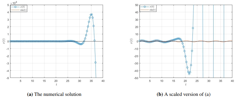
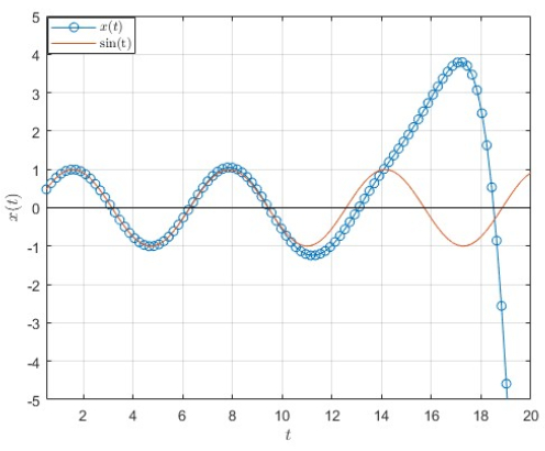
The objective of this work was to provide sufficient conditions for testing the oscillatory performance of solutions of the neutral second-order differential equation with distributed deviation arguments. We derived improved relations that influence the oscillation parameters of the equation under study. We used comparison with lower-order equations and Riccati techniques to derive the oscillation parameters. Comparing our findings with earlier pertinent findings allows us to assess the advancements made in oscillation theory. Furthermore, some numerical solutions for a special case of the equation under study are presented, and the numerical and theoretical results are compared.

| [1] | W. E. Boyce, R. C. DiPrima, D. B. Meade, Elementary Differential Equations and Boundary Value Problems, John Wiley & Sons, 2017. |
| [2] | J. K. Hale, S. M. V. Lunel, Introduction to Functional Differential Equations, Springer Science & Business Media, 2013. |
| [3] | Y. Kuang, Delay Differential Equations with Applications in Population Dynamics, New York: Academic Press, 1993. |
| [4] | S. Saker, Oscillation Theory of Delay Differential and Difference Equations: Second and Third-Orders, LAP Lambert Academic Publishing: Riga, Latvia, 2010. |
| [5] | J. C. F. Sturm, Memoire sur les equations differentielles lineaires du second ordre, J. Math. Pures Appl., 1 (1836), 106–186. |
| [6] |
W. B. Fite, Concerning the zeros of the solutions of certain differential equations, Trans. Am. Math. Soc., 19 (1918), 341–352. https://doi.org/10.1090/S0002-9947-1918-1501107-2 doi: 10.1090/S0002-9947-1918-1501107-2

|
| [7] | R. P. Agarwal, S. R. Grace, D. O'Regan, Oscillation Theory for Second Order Linear, Half-Linear, Superlinear and Sublinear Dynamic Equations, Springer Science & Business Media, 2002. |
| [8] | R. P. Agarwal, S. R. Grace, D. O'Regan, Oscillation Theory for Second Order Dynamic Equations, CRC Press, 2002. |
| [9] | R. P. Agarwal, M. Bohner, W. T. Li, Nonoscillation and Oscillation: Theory for Functional Differential Equations, CRC Press, 2004. |
| [10] | O. Dosly, P. Rehak, Half-Linear Differential Equations, Elsevier, 2005. |
| [11] | I. Győri, G. E. Ladas, Oscillation Theory of Delay Differential Equations: With Applications, Clarendon Press, 1991. https://doi.org/10.1093/oso/9780198535829.001.0001 |
| [12] |
C. Philos, On the existence of nonoscillatory solutions tending to zero at $\infty$ for differential equations with positive delays, Arch. Math., 36 (1981), 168–178. https://doi.org/10.1007/BF01223686 doi: 10.1007/BF01223686
|
| [13] |
S. S. Santra, A. K. Tripathy, On oscillatory first order nonlinear neutral differential equations with nonlinear impulses, J. Appl. Math. Comput., 59 (2018), 257–270. https://doi.org/10.1007/s12190-018-1178-8 doi: 10.1007/s12190-018-1178-8
|
| [14] |
S. S. Santra, D. Baleanu, K. M. Khedher, O. Moaaz, First-order impulsive differential systems: sufficient and necessary conditions for oscillatory or asymptotic behavior, Adv. Differ. Equations, 2021 (2021). https://doi.org/10.1186/s13662-021-03446-1 doi: 10.1186/s13662-021-03446-1
|
| [15] |
E. Tunç, O. Özdemir, Comparison theorems on the oscillation of even order nonlinear mixed neutral differential equations, Math. Methods Appl. Sci., 46 (2022), 631–640. https://doi.org/10.1002/mma.8534 doi: 10.1002/mma.8534
|
| [16] |
T. Li, Y. V. Rogovchenko, On asymptotic behavior of solutions to higher-order sublinear Emden–Fowler delay differential equations, Appl. Math. Lett., 67 (2016), 53–59. https://doi.org/10.1016/j.aml.2016.11.007 doi: 10.1016/j.aml.2016.11.007
|
| [17] |
I. Jadlovská, J. Džurina, J. R. Graef, S. R. Grace, Sharp oscillation theorem for fourth-order linear delay differential equations, J. Inequal. Appl., 2022 (2022). https://doi.org/10.1186/s13660-022-02859-0 doi: 10.1186/s13660-022-02859-0
|
| [18] |
C. Cesarano, O. Moaaz, B. Qaraad, N. A. Alshehri, S. K. Elagan, M. Zakarya, New results for oscillation of solutions of Odd-Order Neutral differential equations, Symmetry, 13 (2021), 1095. https://doi.org/10.3390/sym13061095 doi: 10.3390/sym13061095
|
| [19] | L. Erbe, Q. Kong, B. G. Zhang, Oscillation Theory for Functional Differential Equations, CRC Press, 1994. |
| [20] |
R. P. Agarwal, C. Zhang, T. Li, Some remarks on oscillation of second order neutral differential equations, Appl. Math. Comput., 274 (2015), 178–181. https://doi.org/10.1016/j.amc.2015.10.089 doi: 10.1016/j.amc.2015.10.089
|
| [21] | M. Bohner, S. Grace, I. Jadlovská, Oscillation criteria for second-order neutral delay differential equations, Electron. J. Qual. Theory Differ. Equations, (2017), 1–12. https://doi.org/10.14232/ejqtde.2017.1.60 |
| [22] |
Z. Xu, P. Weng, Oscillation of second order neutral equations with distributed deviating argument, J. Comput. Appl. Math., 202 (2006), 460–477. https://doi.org/10.1016/j.cam.2006.03.001 doi: 10.1016/j.cam.2006.03.001
|
| [23] |
L. Ye, Z. Xu, Oscillation criteria for second order quasilinear neutral delay differential equations, Appl. Math. Comput., 207 (2008), 388–396. https://doi.org/10.1016/j.amc.2008.10.051 doi: 10.1016/j.amc.2008.10.051
|
| [24] |
Z. Han, T. Li, S. Sun, Y. Sun, Remarks on the paper [Appl. Math. Comput. 207 (2009) 388–396], Appl. Math. Comput., 215 (2009), 3998–4007. https://doi.org/10.1016/j.amc.2009.12.006 doi: 10.1016/j.amc.2009.12.006
|
| [25] |
B. Baculíková, J. Džurina, Oscillation theorems for second order neutral differential equations, Comput. Math. Appl., 61 (2010), 94–99. https://doi.org/10.1016/j.camwa.2010.10.035 doi: 10.1016/j.camwa.2010.10.035
|
| [26] |
T. Li, B. Baculíková, J. Džurina, Oscillatory behavior of second-order nonlinear neutral differential equations with distributed deviating arguments, Boundary Value Probl., 2014 (2014). https://doi.org/10.1186/1687-2770-2014-68 doi: 10.1186/1687-2770-2014-68
|
| [27] |
T. Candan, Oscillatory behavior of second order nonlinear neutral differential equations with distributed deviating arguments, Appl. Math. Comput., 262 (2015), 199–203. https://doi.org/10.1016/j.amc.2015.03.134 doi: 10.1016/j.amc.2015.03.134
|
| [28] |
O. Moaaz, R. A. El-Nabulsi, W. Muhsin, O. Bazighifan, Improved oscillation criteria for 2nd-order neutral differential equations with distributed deviating arguments, Mathematics, 8 (2020), 849. https://doi.org/10.3390/math8050849 doi: 10.3390/math8050849
|
| [29] |
O. Moaaz, A. Muhib, S. Owyed, E. E. Mahmoud, A. Abdelnaser, Second-Order neutral differential equations: improved criteria for testing the oscillation, J. Math., 2021 (2021), 1–7. https://doi.org/10.1155/2021/6665103 doi: 10.1155/2021/6665103
|
| [30] |
T. Hassan, O. Moaaz, A. Nabih, M. Mesmouli, A. El-Sayed, New sufficient conditions for oscillation of Second-Order Neutral Delay differential equations, Axioms, 10 (2021), 281. https://doi.org/10.3390/axioms10040281 doi: 10.3390/axioms10040281
|
| [31] |
M. Bohner, S. R. Grace, I. Jadlovská, Sharp results for oscillation of second-order neutral delay differential equations, Electron. J. Qual. Theory Differ. Equations, 2023 (2023), 1–23. https://doi.org/10.14232/ejqtde.2023.1.4 doi: 10.14232/ejqtde.2023.1.4
|
| [32] |
O. Moaaz, E. E. Mahmoud, W. R. Alharbi, Third-Order Neutral Delay Differential equations: new iterative criteria for oscillation, J. Funct. Spaces, 2020 (2020), 1–8. https://doi.org/10.1155/2020/6666061 doi: 10.1155/2020/6666061
|
| [33] |
O. Moaaz, W. Albalawi, Differential equations of the neutral delay type: More efficient conditions for oscillation, AIMS Math., 8 (2023), 12729–12750. https://doi.org/10.3934/math.2023641 doi: 10.3934/math.2023641
|
| [34] |
O. Moaaz, C. Cesarano, B. Almarri, An improved relationship between the solution and its corresponding function in fourth-order neutral differential equations and its applications, Mathematics, 11 (2023), 1708. https://doi.org/10.3390/math11071708 doi: 10.3390/math11071708
|
| [35] |
A. Nabih, O. Moaaz, S. S. Askar, A. M. Alshamrani, E. M. Elabbasy, Fourth-Order neutral differential equation: a modified approach to optimizing monotonic properties, Mathematics, 11 (2023), 4380. https://doi.org/10.3390/math11204380 doi: 10.3390/math11204380
|
| [36] | E. Thandapani, T. Li, On the oscillation of third-order quasi-linear neutral functional differential equations, Arch. Mathematicum, 47 (2011), 181–199. |
| [37] |
C. Zhang, T. Li, B. Sun, E. Thandapani, On the oscillation of higher-order half-linear delay differential equations, Appl. Math. Lett., 24 (2011), 1618–1621. https://doi.org/10.1016/j.aml.2011.04.015 doi: 10.1016/j.aml.2011.04.015
|
| [38] | G. S. Ladde, V. Lakshmikantham, B. G. Zhang, Oscillation Theory of Differential Equations with Deviating Arguments, Marcel Dekker, 1987. |
| [39] |
S. R. Grace, R. P. Agarwal, P. J. Y. Wong, A. Zafer, On the oscillation of fractional differential equations, Fract. Calc. Appl. Anal., 15 (2012), 222–231. https://doi.org/10.2478/s13540-012-0016-1 doi: 10.2478/s13540-012-0016-1
|
| [40] |
D. X. Chen, Oscillation criteria of fractional differential equations, Adv. Differ. Equations, 2012 (2012). https://doi.org/10.1186/1687-1847-2012-33 doi: 10.1186/1687-1847-2012-33
|
Figures(2)
Adeebah Alofee, Ahmed S. Almohaimeed, Osama Moaaz. New iterative criteria for testing the oscillation of solutions of differential equations with distributed deviating arguments[J]. Electronic Research Archive, 2025, 33(6): 3496-3516. doi: 10.3934/era.2025155


 DownLoad: