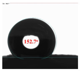
Oil spills pose a significant environmental threat, necessitating the development of efficient and eco-friendly sorbent materials. In this study, a biodegradable cellulose aerogel was successfully synthesized from rambutan peel (RP) waste and evaluated for its diesel oil adsorption performance. The aerogel exhibited ultra-low density (0.027 ± 0.002 g/cm3), high porosity (97.88% ± 0.19%), and excellent hydrophobicity (152.7°). Adsorption experiments demonstrated a maximum diesel oil uptake capacity of 58.8235 g/g under optimal conditions: pH 7, oil concentration of 25 g/L, contact time of 25 s, salinity range of 0‰–35‰, and temperature range of 25–35 ℃. Adsorption equilibrium data were best described by the Langmuir isotherm model (R2 = 0.9974), indicating monolayer adsorption with RL values ranging from 0.0409 to 0.2301 at 25 ℃. Kinetic studies revealed that the pseudo-second-order model provided the best fit (R2 = 0.9998), suggesting that adsorption occurred through both boundary layer diffusion and intraparticle diffusion mechanisms. Thermodynamic analysis confirmed the spontaneity and exothermic nature of the adsorption process. Furthermore, the adsorption mechanism was primarily governed by hydrophobic interactions, van der Waals forces, and hydrogen bonding. Overall, this study highlights the potential of cellulose aerogels derived from agricultural waste as sustainable and highly efficient sorbents for diesel oil removal, offering a promising solution for oil spill remediation in various aquatic environments.
Citation: Nguyen Trinh Trong, Ba Le Huy, Nam Thai Van. Kinetic, isotherm, and thermodynamic studies on diesel oil adsorption by biodegradable cellulose aerogel from rambutan peel waste[J]. AIMS Environmental Science, 2025, 12(3): 373-399. doi: 10.3934/environsci.2025017
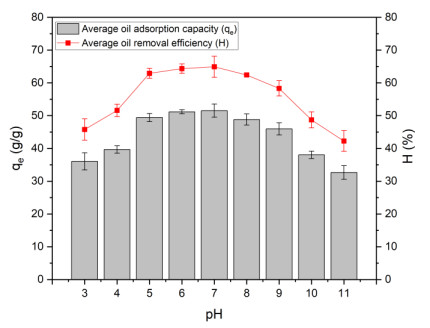
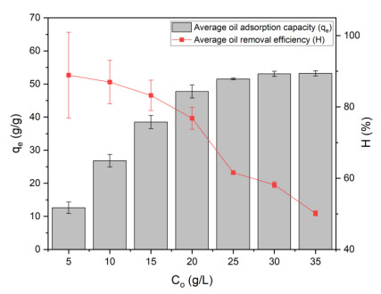
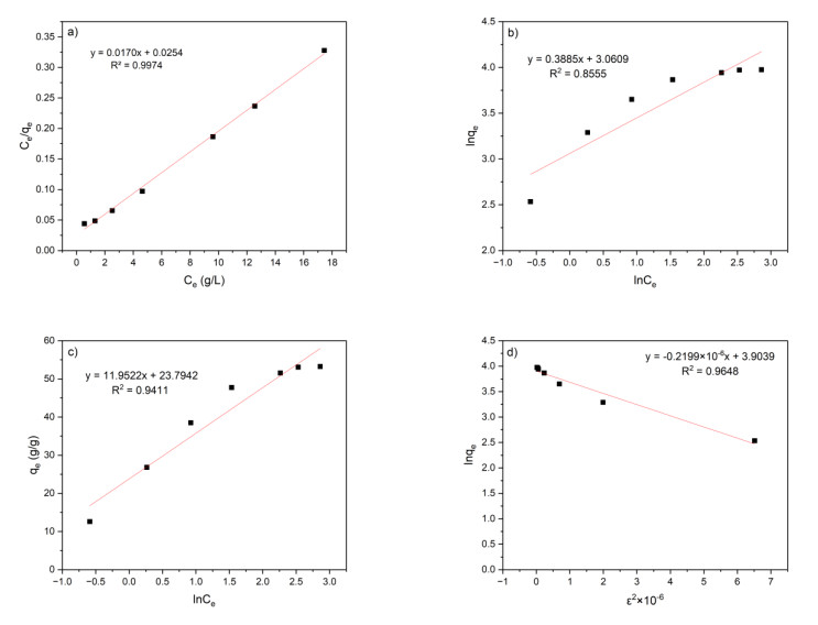
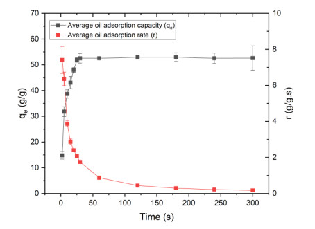
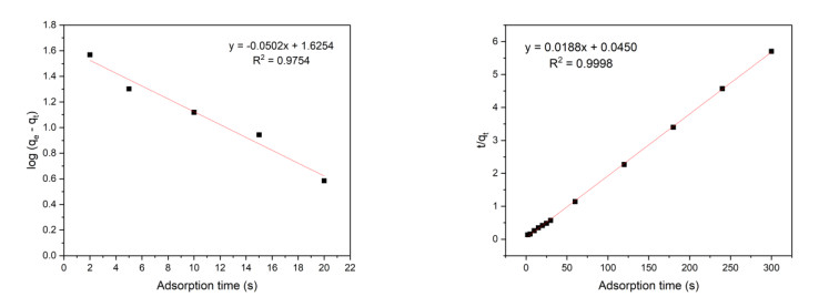
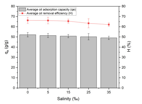
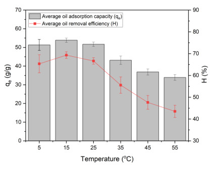
Oil spills pose a significant environmental threat, necessitating the development of efficient and eco-friendly sorbent materials. In this study, a biodegradable cellulose aerogel was successfully synthesized from rambutan peel (RP) waste and evaluated for its diesel oil adsorption performance. The aerogel exhibited ultra-low density (0.027 ± 0.002 g/cm3), high porosity (97.88% ± 0.19%), and excellent hydrophobicity (152.7°). Adsorption experiments demonstrated a maximum diesel oil uptake capacity of 58.8235 g/g under optimal conditions: pH 7, oil concentration of 25 g/L, contact time of 25 s, salinity range of 0‰–35‰, and temperature range of 25–35 ℃. Adsorption equilibrium data were best described by the Langmuir isotherm model (R2 = 0.9974), indicating monolayer adsorption with RL values ranging from 0.0409 to 0.2301 at 25 ℃. Kinetic studies revealed that the pseudo-second-order model provided the best fit (R2 = 0.9998), suggesting that adsorption occurred through both boundary layer diffusion and intraparticle diffusion mechanisms. Thermodynamic analysis confirmed the spontaneity and exothermic nature of the adsorption process. Furthermore, the adsorption mechanism was primarily governed by hydrophobic interactions, van der Waals forces, and hydrogen bonding. Overall, this study highlights the potential of cellulose aerogels derived from agricultural waste as sustainable and highly efficient sorbents for diesel oil removal, offering a promising solution for oil spill remediation in various aquatic environments.

| [1] | Statista Research Department, Global number of oil tanker spills by quantity 1970–2024, 2025. Available from: https://www.statista.com/statistics/268553/number-of-oil-spills-by-oil-tankers-since-1970/. |
| [2] |
Zamparas M, Tzivras D, Dracopoulos V, et al. (2020) Application of sorbents for oil spill cleanup focusing on natural-based modified materials: A review. Molecules 25: 4522. https://doi.org/10.3390/molecules25194522 doi: 10.3390/molecules25194522

|
| [3] |
El-Din GA, Amer AA, Malsh G, et al. (2018) Study on the use of banana peels for oil spill removal. Alex Eng J 57: 2061–2068. https://doi.org/10.1016/j.aej.2017.05.020 doi: 10.1016/j.aej.2017.05.020
|
| [4] |
Chen X, Yang S, Chen T, et al. (2022) Highly mesoporous and compressible sugarcane aerogel via top-down nanotechnology as effective and reusable oil absorbents. Cellulose 30: 1–16. https://doi.org/10.1007/s10570-022-04949-0 doi: 10.1007/s10570-022-04949-0
|
| [5] |
Banerjee SS, Joshi MV, Jayaram RV (2006) Treatment of oil spill by sorption technique using fatty acid grafted sawdust. Chemosphere 64: 1026–1031. https://doi.org/10.1016/j.chemosphere.2006.01.065 doi: 10.1016/j.chemosphere.2006.01.065
|
| [6] |
Long LY, Weng YX, Wang YZ (2018) Cellulose aerogels: Synthesis, applications, and prospects. Polymers 10: 623. https://doi.org/10.3390/polym10060623 doi: 10.3390/polym10060623
|
| [7] |
Zhen L, Thai QB, Nguyen TX, et al. (2019) Recycled cellulose aerogels from paper waste for a heat insulation design of canteen bottles. Fluids 4: 174. https://doi.org/10.3390/fluids4030174 doi: 10.3390/fluids4030174
|
| [8] |
Jian L, Caichao W, Yun L, et al. (2014) Fabrication of cellulose aerogel from wheat straw with strong absorptive capacity. Front Agric Sci Eng 1: 46–52. https://doi.org/10.15302/J-FASE-2014004 doi: 10.15302/J-FASE-2014004
|
| [9] |
Yin T, Zhang X, Liu X, et al. (2016) Cellulose-based aerogel from Eichhornia crassipes as an oil superabsorbent. RSC Adv 6: 98563–98570. https://doi.org/10.1039/C6RA22950F doi: 10.1039/C6RA22950F
|
| [10] |
Zhang X, Kwek L, Le D, et al. (2019) Fabrication and properties of hybrid coffee-cellulose aerogels from spent coffee grounds. Polymers 11: 1942. https://doi.org/10.3390/polym11121942 doi: 10.3390/polym11121942
|
| [11] |
Li W, Li Z, Wang W, et al. (2021) Green approach to facilely design hydrophobic aerogel directly from bagasse. Ind Crops Prod 172: 113957. https://doi.org/10.1016/j.indcrop.2021.113957 doi: 10.1016/j.indcrop.2021.113957
|
| [12] |
Yen TD, Nga HND, Phuong TXN, et al. (2022) Green fabrication of bio-based aerogels from coconut fibers for wastewater treatment. J Porous Mat 29: 1–14. https://doi.org/10.1007/s10934-022-01257-7 doi: 10.1007/s10934-022-01257-7
|
| [13] |
Chung VN, Nguyen TS, Huynh KPH, et al. (2022) Fabrication of cellulose aerogel from waste paper and banana peel for water treatment. Chem Eng Trans 97: 337–342. https://doi.org/10.3303/CET2297057 doi: 10.3303/CET2297057
|
| [14] | Mai TN, Luu TP, Nga DNH, et al. (2019) Fabrication of cotton aerogels and its application in water treatment, Proceedings of the 12th Regional Conference on Chemical Engineering, 85–90. |
| [15] |
Dong C, Hu Y, Zhu Y, et al. (2022) Fabrication of textile waste fibers aerogels with excellent oil/organic solvent adsorption and thermal properties. Gels 8: 684. https://doi.org/10.3390/gels8100684 doi: 10.3390/gels8100684
|
| [16] |
Nguyen TT, Le Tan PH, Ngoc DN, et al. (2024) Optimizing the synthesis conditions of aerogels based on cellulose fiber extracted from rambutan peel using response surface methodology. AIMS Environ Sci 11: 276–292. https://doi.org/10.3934/environsci.2024028 doi: 10.3934/environsci.2024028
|
| [17] |
Nguyen TTV, Tri N, Tran BA, et al. (2021) Synthesis, characteristics, oil adsorption, and thermal insulation performance of cellulosic aerogel derived from water hyacinth. ACS Omega 6: 26130–26139. https://doi.org/10.1021/acsomega.1c03137 doi: 10.1021/acsomega.1c03137
|
| [18] |
Nga HND, Thao PL, Quoc BT, et al. (2019) Advanced fabrication and application of pineapple aerogels from agricultural waste. Mater Technol 35: 1–8. https://doi.org/10.1080/10667857.2019.1688537 doi: 10.1080/10667857.2019.1688537
|
| [19] |
Meng Y, Wang X, Wu Z, et al. (2015) Optimization of cellulose nanofibrils carbon aerogel fabrication using response surface methodology. Eur Polym J 73: 137–148. https://doi.org/10.1016/j.eurpolymj.2015.10.007 doi: 10.1016/j.eurpolymj.2015.10.007
|
| [20] |
Thai QB, Nguyen ST, Ho DK, et al. (2019) Cellulose-based aerogels from sugarcane bagasse for oil spill-cleaning and heat insulation applications. Carbohyd Polym 228: 115365. https://doi.org/10.1016/j.carbpol.2019.115365 doi: 10.1016/j.carbpol.2019.115365
|
| [21] |
Shi G, Qian Y, Tan F, et al. (2019) Controllable synthesis of pomelo peel-based aerogel and its application in adsorption of oil/organic pollutants. Roy Soc Open Sci 6: 181823. https://doi.org/10.1098/rsos.181823 doi: 10.1098/rsos.181823
|
| [22] |
Ahmad MA, Alrozi R (2011) Optimization of rambutan peel based activated carbon preparation conditions for Remazol Brilliant Blue R removal. J Chem Eng 168: 280–285. https://doi.org/10.1016/j.cej.2011.01.005 doi: 10.1016/j.cej.2011.01.005
|
| [23] |
D. Ahuja, S. Dhiman, G. Rattan, et al. (2021) Superhydrophobic modification of cellulose sponge fabricated from discarded jute bags for oil water separation. J Environ Chem Eng 9: 105063. https://doi.org/10.1016/j.jece.2021.105063 doi: 10.1016/j.jece.2021.105063
|
| [24] |
Loh J, Goh X, Nguyen P, et al. (2022) Advanced aerogels from wool waste fibers for oil spill cleaning applications. J Environ Polym Degr 30: 1–14. https://doi.org/10.1007/s10924-021-02234-y doi: 10.1007/s10924-021-02234-y
|
| [25] |
Kumar G, Dora DTK, Jadav D, et al. (2021) Utilization and regeneration of waste sugarcane bagasse as a novel robust aerogel as an effective thermal, acoustic insulator, and oil adsorbent. J Clean Prod 298: 126744. https://doi.org/10.1016/j.jclepro.2021.126744 doi: 10.1016/j.jclepro.2021.126744
|
| [26] |
Wang H, Chen X, Chen B, et al. (2024) Development of a spiropyran-assisted cellulose aerogel with switchable wettability as oil sorbent for oil spill cleanup. Sci Total Environ 923: 171451. https://doi.org/10.1016/j.scitotenv.2024.171451 doi: 10.1016/j.scitotenv.2024.171451
|
| [27] |
Nguyen S, Feng J, Ng S, et al. (2014) Advanced thermal insulation and absorption properties of recycled cellulose aerogels. Colloid Surface A 445: 128–134. https://doi.org/10.1016/j.colsurfa.2014.01.015 doi: 10.1016/j.colsurfa.2014.01.015
|
| [28] |
Du TT, Son TN, Duc Do N, et al. (2020) Green aerogels from rice straw for thermal, acoustic insulation and oil spill cleaning applications. Mater Chem Phys 253: 123363. https://doi.org/10.1016/j.matchemphys.2020.123363 doi: 10.1016/j.matchemphys.2020.123363
|
| [29] |
Luu TP, Do NHN, Chau NDQ, et al. (2020) Morphology control and advanced properties of bio-aerogels from pineapple leaf waste. Chem Eng Trans 78: 433–438. https://doi.org/10.3303/CET2078073 doi: 10.3303/CET2078073
|
| [30] |
Nga DNH, Luu TP, Thai QB, et al. (2019) Heat and sound insulation applications of pineapple aerogels from pineapple waste. Mater Chem Phys 242: 122267. https://doi.org/10.1016/j.matchemphys.2019.122267 doi: 10.1016/j.matchemphys.2019.122267
|
| [31] |
Nguyen ST, Feng J, Le NT (2013) Cellulose aerogel from paper waste for crude oil spill cleaning. Ind Eng Chem Res 52: 18386–18391. https://doi.org/10.1021/ie4032567 doi: 10.1021/ie4032567
|
| [32] |
Peng D, Zhao J, Liang X, et al. (2023) Corn stalk pith-based hydrophobic aerogel for efficient oil sorption. J Hazard Mater 448: 130954. https://doi.org/10.1016/j.jhazmat.2023.130954 doi: 10.1016/j.jhazmat.2023.130954
|
| [33] |
Lang D, Zhang C, Qian Q, et al. (2023) Oil absorption stability of modified cellulose porous materials with super compressive strength in the complex environment. Cellulose 30: 7745–7762. https://doi.org/10.1007/s10570-023-05322-5 doi: 10.1007/s10570-023-05322-5
|
| [34] |
Xiao S, Gao R, Lu Y, et al. (2015) Fabrication and characterization of nanofibrillated cellulose and its aerogels from natural pine needles. Carbohyd Polym 119. https://doi.org/10.1016/j.carbpol.2014.11.041 doi: 10.1016/j.carbpol.2014.11.041
|
| [35] |
Panda D, Gangawane KM (2023) Recycled cellulose–silica hybrid aerogel for effective oil adsorption: optimization and kinetics study. Sādhanā 48: 110. https://doi.org/10.1007/s12046-023-02161-9 doi: 10.1007/s12046-023-02161-9
|
| [36] |
Dilamian M, Noroozi B (2021) Rice straw agri-waste for water pollutant adsorption: Relevant mesoporous super hydrophobic cellulose aerogel. Carbohyd Polym 251: 117016. https://doi.org/10.1016/j.carbpol.2020.117016 doi: 10.1016/j.carbpol.2020.117016
|
| [37] |
Zhai Y, Yuan X, Weber CC, et al. (2024) Review of plant cellulose-based aerogel materials for oil/water mixture separation. J Environ Chem Eng 12: 113716. https://doi.org/10.1016/j.jece.2024.113716 doi: 10.1016/j.jece.2024.113716
|
| [38] |
Penjumras P, Rahman RA, Talib RA, et al. (2014) Extraction and Characterization of Cellulose from Durian Rind. Agric Agric Sci Procedia 2: 237–243. https://doi.org/10.1016/j.aaspro.2014.11.034 doi: 10.1016/j.aaspro.2014.11.034
|
| [39] |
Conrad A, Saona LR, Mcpherson B, et al. (2014) Identification of Quercus agrifolia (coast live oak) resistant to the invasive pathogen Phytophthora ramorum in native stands using Fourier-transform infrared (FT-IR) spectroscopy. Front Plant Sci 5: 521. https://doi.org/10.3389/fpls.2014.00521 doi: 10.3389/fpls.2014.00521
|
| [40] |
Kumar N, Pruthi V (2015) Structural elucidation and molecular docking of ferulic acid from Parthenium hysterophorus possessing COX-2 inhibition activity. 3 Biotech 5: 541–551. https://doi.org/10.1007/s13205-014-0253-6 doi: 10.1007/s13205-014-0253-6
|
| [41] |
Chau NDQ, Nghiem TTN, Doan HLX, et al. (2020) Advanced fabrication and applications of cellulose acetate aerogels from cigarette butts. Mater Trans 61: 1550–1554. https://doi.org/10.2320/matertrans.MT-MN2019009 doi: 10.2320/matertrans.MT-MN2019009
|
| [42] |
R. Lu, W. Gan, B. Wu, et al. (2005) C−H stretching vibrations of methyl, methylene and methine groups at the vapor/alcohol (n = 1−8) interfaces. J Phys Chem B 109: 14118–29. https://doi.org/10.1021/jp051565q doi: 10.1021/jp051565q
|
| [43] |
Lv P, Almeida G, Perré P (2015) TGA-FTIR analysis of torrefaction of Lignocellulosic components (cellulose, xylan, lignin) in isothermal conditions over a wide range of time durations. BioResources 10: 4239–4251. https://doi.org/10.15376/biores.10.3.4239-4251 doi: 10.15376/biores.10.3.4239-4251
|
| [44] |
Anusha YG, Machado AA, Mulky L (2023) A comparative study of treatment methods of raw sugarcane bagasse for adsorption of oil and diesel. Water Air Soil Pollut 234: 213. https://doi.org/10.1007/s11270-023-06210-1 doi: 10.1007/s11270-023-06210-1
|
| [45] |
Atoufi Z, Ciftci GC, Reid MS, et al. (2022) Green ambient-dried aerogels with a facile pH-tunable surface charge for adsorption of cationic and anionic contaminants with high selectivity. Biomacromolecules 23: 4934–4947. https://doi.org/10.1021/acs.biomac.2c01142 doi: 10.1021/acs.biomac.2c01142
|
| [46] |
Sokker HH, El-Sawy NM, Hassan MA, et al. (2011) Adsorption of crude oil from aqueous solution by hydrogel of chitosan based polyacrylamide prepared by radiation induced graft polymerization. J Hazard Mater 190: 359–365. https://doi.org/10.1016/j.jhazmat.2011.03.055 doi: 10.1016/j.jhazmat.2011.03.055
|
| [47] |
Mo L, Pang H, Tan Y, et al. (2019) 3D multi-wall perforated nanocellulose-based polyethylenimine aerogels for ultrahigh efficient and reversible removal of Cu(Ⅱ) ions from water. J Chem Eng 378: 122157. https://doi.org/10.1016/j.cej.2019.122157 doi: 10.1016/j.cej.2019.122157
|
| [48] | Khanjanzadeh H, et al. (2018) Surface chemical functionalization of cellulose nanocrystals by 3-aminopropyltriethoxysilane. Int J Biol Macromol 106: 1288–1296. |
| [49] | Salisu ZM, Hasan DB, Liman YG, et al. (2022) Critical studies on the kinetics, isotherms and activation energy of sorption phenomenon for optimized Kenaf Shive sorbent in crude oil/seawater system, In: Biodegradation Technology of Organic and Inorganic Pollutants, IntechOpen, 1–18. https://doi.org/10.5772/intechopen.98658 |
| [50] |
Nguyen TTV, Yang GX, Phan AN, et al. (2022) Insights into the effects of synthesis techniques and crosslinking agents on the characteristics of cellulosic aerogels from Water Hyacinth. RSC Adv 12: 19225–19231. https://doi.org/10.1039/D2RA02944H doi: 10.1039/D2RA02944H
|
| [51] |
Paulauskiene T, Uebe J, Karasu A, et al. (2020) Investigation of cellulose-based aerogels for oil spill removal. Water Air Soil Poll 231: 424. https://doi.org/10.1007/s11270-020-04799-1 doi: 10.1007/s11270-020-04799-1
|
| [52] |
Wozniak AB, Piontek JC, Wiercińska AN, et al. (2022) Adsorption of organic compounds on adsorbents obtained with the use of microwave heating. Materials 15: 5664. https://doi.org/10.3390/ma15165664 doi: 10.3390/ma15165664
|
| [53] |
Nandiyanto ABD, Girsang GCS, Maryanti R, et al. (2020) Isotherm adsorption characteristics of carbon microparticles prepared from pineapple peel waste. Commun Sci Technol 5: 31–39. https://doi.org/10.21924/cst.5.1.2020.176 doi: 10.21924/cst.5.1.2020.176
|
| [54] |
El-Harby NF, Ibrahim SMA, Mohamed NA (2017) Adsorption of Congo red dye onto antimicrobial terephthaloyl thiourea cross-linked chitosan hydrogels. Water Sci Technol 76: 2719–2732. https://doi.org/10.2166/wst.2017.442 doi: 10.2166/wst.2017.442
|
| [55] |
Zhou L, Zhai S, Chen Y, et al. (2019) Anisotropic cellulose nanofibers/polyvinyl alcohol/graphene aerogels fabricated by directional freeze-drying as effective oil adsorbents. Polymers 11: 712. https://doi.org/10.3390/polym11040712 doi: 10.3390/polym11040712
|
| [56] |
Feng J, Nguyen S, Fan Z, et al. (2015) Advanced fabrication and oil absorption properties of super-hydrophobic recycled cellulose aerogels. Chem Eng J 270: 168–175. https://doi.org/10.1016/j.cej.2015.02.034 doi: 10.1016/j.cej.2015.02.034
|
| [57] |
Vu P, Doan T, Tu G, et al. (2022) A novel application of cellulose aerogel composites from pineapple leaf fibers and cotton waste: Removal of dyes and oil in wastewater. J Porous Mat 29: 1137–1147. https://doi.org/10.21203/rs.3.rs-1102952/v1 doi: 10.21203/rs.3.rs-1102952/v1
|
| [58] | Phương NTX (2024) Synthesis of cellulose aerogel from coir fiber for the application in treating some organic dyes and lubricating oil, Ph.D. Dissertation, Ho Chi Minh City University of Technology, Vietnam. |
| [59] |
Urgel JJDT, Briones JMA, Diaz EB, et al. (2024) Batch adsorption of diesel oil in water using saba banana peel biochar immobilized in teabags. J Appl Eng Sci 71: 59. https://doi.org/10.1186/s44147-024-00398-7 doi: 10.1186/s44147-024-00398-7
|
| [60] |
Zhang C, Chen GH, Lang DN, et al. (2024) Superhydrophobic cellulose-nanofiber aerogels from waste cotton stalks for superior oil–water and emulsion separation. Cellulose 31: 8519–8538. https://doi.org/10.1007/s10570-024-06118-x doi: 10.1007/s10570-024-06118-x
|
| [61] |
Galblaub OA, Shaykhiev IG, Stepanova SV, et al. (2016) Oil spill cleanup of water surface by plant-based sorbents: Russian practices. Process Saf Environ 101: 88–92. https://doi.org/10.1016/j.psep.2015.11.002 doi: 10.1016/j.psep.2015.11.002
|
| [62] |
Bayat A, Aghamiri SF, Moheb A, et al. (2005) Oil spill cleanup from sea water by sorbent materials. Chem Eng Technol 28: 1525–1528. https://doi.org/10.1002/ceat.200407083 doi: 10.1002/ceat.200407083
|
| [63] | Phương HT (2018) Study on the Synthesis and Modification of Nano Silica Materials for Oil Recovery Applications, Ph.D. Dissertation, Hanoi University of Science and Technology, Vietnam. |
| [64] |
Omer AM, Khalifa RE, Tamer TM, et al. (2020) Kinetic and thermodynamic studies for the sorptive removal of crude oil spills using a low-cost chitosan-poly (butyl acrylate) grafted copolymer, Desalin Water Treat 192: 213–225. https://doi.org/10.5004/dwt.2020.25704 doi: 10.5004/dwt.2020.25704
|
| [65] |
Mahmoud MA, Tayeb AM, Daher AM, et al. (2022) Adsorption study of oil spill cleanup from sea water using natural sorbent. Chem Data Collect 41: 100896. https://doi.org/10.1016/j.cdc.2022.100896 doi: 10.1016/j.cdc.2022.100896
|
| [66] |
Lv N, Wang X, Peng S, et al. (2018) Superhydrophobic/superoleophilic cotton-oil absorbent: Preparation and its application in oil/water separation. RSC Adv 8: 30257–30264. https://doi.org/10.1039/c8ra05420g doi: 10.1039/c8ra05420g
|
| [67] | Zhou X, Yu X, Maimaitiniyazi R, et al. (2024) Discussion on the thermodynamic calculation and adsorption spontaneity re Ofudje et al. (2023). Heliyon 10: e28188. https://doi.org/10.1016/j.heliyon.2024.e28188 |
| [68] |
Nazifa TH, Hadibarata T, Yuniarto A, et al. (2019) Equilibrium, kinetic and thermodynamic analysis petroleum oil adsorption from aqueous solution by magnetic activated carbon. IOP Conf Ser: Mater Sci Eng 495: 012060. https://doi.org/10.1088/1757-899X/495/1/012060 doi: 10.1088/1757-899X/495/1/012060
|
| [69] |
Liu G, Wang N, Zhou J, et al. (2015) Microbial preparation of magnetite/reduced graphene oxide nanocomposites for the removal of organic dyes from aqueous solutions. RSC Adv 5: 95857–95865. https://doi.org/10.1039/C5RA18136D doi: 10.1039/C5RA18136D
|
| [70] |
Hammood A, Khwedem A, Zaidan A, et al. (2023) Thermodynamics study of adsorption of oil hydrocarbons from aqueous solutions onto the porcelanite surface. J Kufa Chem Sci 2: 178–188. https://doi.org/10.36329/jkcm/2022/v2.i9.13293 doi: 10.36329/jkcm/2022/v2.i9.13293
|
| [71] | Masterton WL, Slowinski EJ, Stanitski CL (1983) Chemical principles: Alternate edition with a qualitative analysis supplement, New York: CBS College Publishing/Saunders College Publishing. |
| [72] |
El-Araby HA, Ibrahim AMMA, Mangood AH (2017) Sesame husk as adsorbent for Copper (Ⅱ) ions removal from aqueous solution. J Geosci Environ Pro 5: 109–152. https://doi.org/10.4236/gep.2017.57011 doi: 10.4236/gep.2017.57011
|
| [73] |
Ifelebuegu AO, Johnson A (2017) Nonconventional low-cost cellulose- and keratin-based biopolymeric sorbents for oil/water separation and spill cleanup: A review. Crit Rev Env Sci Tec 47: 964–1001. https://doi.org/10.1080/10643389.2017.1318620 doi: 10.1080/10643389.2017.1318620
|
| [74] |
Sabir S (2015) Approach of cost-effective adsorbents for oil removal from oily water. Crit Rev Env Sci Tec 45: 1916–1945. https://doi.org/10.1080/10643389.2014.1001143 doi: 10.1080/10643389.2014.1001143
|
| [75] |
Wang S, Peng XW, Zhong LX, et al. (2015) An ultralight, elastic, cost-effective, and highly recyclable superabsorbent from microfibrillated cellulose fibers for oil spillage cleanup. J Mater Chem A 3: 8772–8781. https://doi.org/10.1039/C4TA07057G doi: 10.1039/C4TA07057G
|
| [76] |
Huang J, Yan Z (2018) Adsorption mechanism of oil by resilient graphene aerogels from oil–water emulsion, Langmuir 34: 1890–1898. https://doi.org/10.1021/acs.langmuir.7b03866 doi: 10.1021/acs.langmuir.7b03866
|
Figures(14) / Tables(8)

Nguyen Trinh Trong, Ba Le Huy, Nam Thai Van. Kinetic, isotherm, and thermodynamic studies on diesel oil adsorption by biodegradable cellulose aerogel from rambutan peel waste[J]. AIMS Environmental Science, 2025, 12(3): 373-399. doi: 10.3934/environsci.2025017


 DownLoad: