For the wood moisture content (MC) detection engineering problem by planar capacitive sensors, a high accuracy is required. To meet this demand, we constructed a mathematical model in this paper, as this is an inverse problem in the multi-physics fields. Furthermore, we proposed a new numerical method with high accuracy, which is called the multiple varying bounds integral method. We applied this numerical method to establish a high accuracy and compact numerical scheme for solving this model. Because the unknown function is continuous in some physical fields and discontinuous in others, we needed to use different numerical methods to construct numerical schemes in these fields. For example, we used the multiple varying bounds integral (MVBI) method and interpolation methods. Next, based on the results of the numerical experiments, a regression model was established between capacitance and the dielectric constant of wood. The results indicated that the larger the value of dielectric constant, the larger the value of capacitance. This is consistent with the physical principle. Moreover, the determination coefficient $ R^{2} $ of the regression model was greater than 0.91. Additionally, the confidence degree exceeded 0.99, which implies that the reliability of the regression model is strong. This indicates that the regression model shows a high goodness of fit and high confidence degree.
Citation: Cui Guo, Yixue Wang, Haibin Wang, Xiongbo Zheng, Bin Zhao. Non-destructive test method of wood moisture content based on multiple varying bounds integral numerical method[J]. Electronic Research Archive, 2025, 33(4): 2246-2274. doi: 10.3934/era.2025098
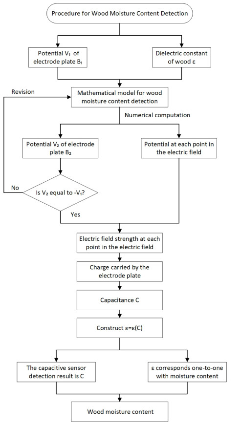
For the wood moisture content (MC) detection engineering problem by planar capacitive sensors, a high accuracy is required. To meet this demand, we constructed a mathematical model in this paper, as this is an inverse problem in the multi-physics fields. Furthermore, we proposed a new numerical method with high accuracy, which is called the multiple varying bounds integral method. We applied this numerical method to establish a high accuracy and compact numerical scheme for solving this model. Because the unknown function is continuous in some physical fields and discontinuous in others, we needed to use different numerical methods to construct numerical schemes in these fields. For example, we used the multiple varying bounds integral (MVBI) method and interpolation methods. Next, based on the results of the numerical experiments, a regression model was established between capacitance and the dielectric constant of wood. The results indicated that the larger the value of dielectric constant, the larger the value of capacitance. This is consistent with the physical principle. Moreover, the determination coefficient $ R^{2} $ of the regression model was greater than 0.91. Additionally, the confidence degree exceeded 0.99, which implies that the reliability of the regression model is strong. This indicates that the regression model shows a high goodness of fit and high confidence degree.

| [1] |
M. Broda, S. F. Curling, M. Frankowski, The effect of the drying method on the cell wall structure and sorption properties of waterlogged archaeological wood, Wood Sci. Technol., 55 (2021), 971–989. https://doi.org/10.1007/s00226-021-01294-6 doi: 10.1007/s00226-021-01294-6

|
| [2] |
Z. B. He, J. Qian, L. J. Qu, Z. Y. Wang, S. L. Yi, Simulation of moisture transfer during wood vacuum drying, Results Phys., 12 (2019), 1299–1303. https://doi.org/10.1016/j.rinp.2019.01.017 doi: 10.1016/j.rinp.2019.01.017
|
| [3] |
O. E. Özkan, Effects of cryogenic temperature on some mechanical properties of beech (Fagus orientalis Lipsky) wood, Eur. J. Wood Wood Prod., 79 (2021), 417–421. https://doi.org/10.1007/s00107-020-01639-1 doi: 10.1007/s00107-020-01639-1
|
| [4] |
L. Rostom, S. Caré, D. Courtier‐Murias, Analysis of water content in wood material through 1D and 2D H-1 NMR relaxometry: Application to the determination of the dry mass of wood, Magn. Reson. Chem., 59 (2021), 614–627. https://doi.org/10.1002/mrc.5125 doi: 10.1002/mrc.5125
|
| [5] | M. D. Ji, C. S. Gui, J. W. Ao, Y. F. Shen, J. Z. Zhao, J. J. Fu, Analysis of innovation trends of Chinese wood flooring industry (in Chinese), China Wood-Based Panels, 28 (2021), 7–9. |
| [6] | M. Li, D. Chen, K. Tian, J. M. He, Y. H. She, Experimental study on cracking load of wood membersunder different moisture content (in Chinese), For. Eng., 38 (2022), 69–81. |
| [7] |
X. Xu, H. Chen, B. H. Fei, W. F. Zhang, T. H. Zhong, Effects of age, particle size and moisture content on physical and mechanical properties of moso bamboo non-glue bonded composites (in Chinese), J. For. Eng., 8 (2023), 30–37. https://doi.org/10.13360/j.issn.2096-1359.202204036 doi: 10.13360/j.issn.2096-1359.202204036
|
| [8] |
P. Dietsch, S. Franke, B. Franke, A. Gamper, S. Winter, Methods to determine wood moisture content and their applicability in monitoring concepts, J. Civ. Struct. Health Monit., 5 (2015), 115–127. https://doi.org/10.1007/s13349-014-0082-7 doi: 10.1007/s13349-014-0082-7
|
| [9] |
L. Martin, H. Cochard, S. Mayr, E. Badel, Using electrical resistivity tomography to detect wetwood and estimate moisture content in silver fir, Ann. For. Sci., 78 (2021), 65. https://doi.org/10.1007/s13595-021-01078-9 doi: 10.1007/s13595-021-01078-9
|
| [10] |
J. Van Blokland, S. Adamopoulos, Electrical resistance characteristics of thermally modified wood, Eur. J. Wood Wood Prod., 80 (2022), 749–752. https://doi.org/10.1007/s00107-022-01813-7 doi: 10.1007/s00107-022-01813-7
|
| [11] |
W. R. N. Edwards, P. G. Jarvis, A method for measuring radial differences in water content of intact tree stems by attenuation of gamma radiation, Plant Cell Environ., 6 (1983), 255–260. https://doi.org/10.1111/1365-3040.ep11587650 doi: 10.1111/1365-3040.ep11587650
|
| [12] |
A. V. Batranin, S. L. Bondarenko, M. A. Kazaryan, A. A. Krasnykh, I. A. Miloichikova, S. V. Smirnov, et al., Evaluation of the effect of moisture content in the wood sample structure on the quality of tomographic X-Ray studies of tree rings of stem wood, Bull. Lebedev Phys. Inst., 46 (2019), 16–18. https://doi.org/10.3103/S1068335619010056 doi: 10.3103/S1068335619010056
|
| [13] |
P. A. Penttilä, M. Altgen, N. Carl, P. van Der Linden, I. Morfin, M. Österberg, et al., Moisture-related changes in the nanostructure of woods studied with X-ray and neutron scattering, Cellulose, 27 (2020), 71–87. https://doi.org/10.1007/s10570-019-02781-7 doi: 10.1007/s10570-019-02781-7
|
| [14] |
R. X. Qin, H. D. Xu, N. Z. Chen, Z. L. Zhen, J. D. Wei, The correlation between wood moisture content and dielectric constant based on dielectric spectroscopy (in Chinese), J. Cent. South Univ. For. Technol., 42 (2022), 162–169. https://doi.org/10.14067/j.cnki.1673-923x.2022.03.017 doi: 10.14067/j.cnki.1673-923x.2022.03.017
|
| [15] | W. Y. Tang, X. L. Zhang, Sensors, 6th edition, China Machine Press, Beijing, 2021. |
| [16] |
V. T. H. Tham, T. Inagaki, S. Tsuchikawa, A new approach based on a combination of capacitance and near-infrared spectroscopy for estimating the moisture content of timber, Wood Sci. Technol., 53 (2019), 579–599. https://doi.org/10.1007/s00226-019-01077-0 doi: 10.1007/s00226-019-01077-0
|
| [17] |
S. K. Korkua, S. Sakphrom, Low-cost capacitive sensor for detecting palm-wood moisture content in real-time, Heliyon, 6 (2020), e04555. https://doi.org/10.1016/j.heliyon.2020.e04555 doi: 10.1016/j.heliyon.2020.e04555
|
| [18] |
H. Li, M. Perrin, F. Eyma, X. Jacob, V. Gibiat, Moisture content monitoring in glulam structures by embedded sensors via electrical methods, Wood Sci. Technol., 52 (2018), 733–752. https://doi.org/10.1007/s00226-018-0989-y doi: 10.1007/s00226-018-0989-y
|
| [19] |
Z. Wang, X. M. Wang, Z. J. Chen, Water states and migration in Xinjiang poplar and Mongolian Scotch pine monitored by TD-NMR during drying, Holzforschung, 72 (2018), 113–123. https://doi.org/10.1515/hf-2017-0033 doi: 10.1515/hf-2017-0033
|
| [20] | D. Wu, Several Studies on Finite Volume Methods for Diffusion Problems (in Chinese), Ph.D thesis, Jilin University, 2023. |
| [21] | X. Liu, Research on Polyhedral Mesh Quality Based on Finite Volumn Method (in Chinese), Ph.D thesis, Chongqing University of Posts and Telecommunications, 2022. https://doi.org/10.27675/d.cnki.gcydx.2022.001125 |
| [22] |
U. Ahmed, D. S. Mashat, D. A. Maturi, Finite volume method for a time-dependent convection-diffusion-reaction equation with small parameters, Int. J. Differ. Equations, 2022 (2022), 3476309. https://doi.org/10.1155/2022/3476309 doi: 10.1155/2022/3476309
|
| [23] |
Y. S. Luo, X. L. Li, C. Guo, Fourth-order compact and energy conservative scheme for solving nonlinear Klein-Gordon equation, Numer. Methods Partial Differ. Equations, 33 (2017), 1283–1304. https://doi.org/10.1002/num.22143 doi: 10.1002/num.22143
|
| [24] |
C. Guo, W. J. Xue, Y. L. Wang, Z. X. Zhang, A new implicit nonlinear discrete scheme for Rosenau-Burgers equation based on multiple integral finite volume method, AIP Adv., 10 (2020), 045125. https://doi.org/10.1063/1.5142004 doi: 10.1063/1.5142004
|
| [25] |
C. Guo, F. Li, W. Zhang, Y. S. Luo, A conservative numerical scheme for rosenau-rlw equation based on multiple integral finite volume method, Bound. Value Probl., 2019 (2019), 168. https://doi.org/10.1186/s13661-019-1273-2 doi: 10.1186/s13661-019-1273-2
|
| [26] |
C. Guo, Y. Wang, Y. S. Luo, A conservative and implicit second-order nonlinear numerical scheme for the rosenau-kdv equation, Mathematics, 9 (2021), 1183. https://doi.org/10.3390/math9111183 doi: 10.3390/math9111183
|
| [27] |
J. N. Wu, C. Guo, B. Y. Fan, X. B. Zheng, X. L. Li, Y. X. Wang, Two high-precision compact schemes for the dissipative symmetric regular long wave (SRLW) equation by multiple varying bounds integral method, AIP Adv., 14 (2024), 125009. https://doi.org/10.1063/5.0233771 doi: 10.1063/5.0233771
|
| [28] | Y. S. Luo, C. Guo, Q. S. Liu, S. Liang, S. G. Liu, Mathematical model and its application of the planar capacitance sensor under non-uniform and non-symmetrical conditions (in Chinese), Chin. J. Eng. Math., 30 (2013), 317–328. |
| [29] |
D. Chalishajar, D. Kasinathan, R. Kasinathan, Viscoelastic Kelvin–Voigt model on Ulam–Hyer's stability and T-controllability for a coupled integro fractional stochastic systems with integral boundary conditions via integral contractors, Chaos Solitons Fractals, 191 (2025), 115785. https://doi.org/10.1016/j.chaos.2024.115785 doi: 10.1016/j.chaos.2024.115785
|
| [30] | C. Guo, Research on Mathematical Model and Algorithm of Capacitance Sensor Used to Detect Wood Moisture Content (in Chinese), Ph.D thesis, Harbin Engineering University, 2014. |


Figures(14) / Tables(2)
Cui Guo, Yixue Wang, Haibin Wang, Xiongbo Zheng, Bin Zhao. Non-destructive test method of wood moisture content based on multiple varying bounds integral numerical method[J]. Electronic Research Archive, 2025, 33(4): 2246-2274. doi: 10.3934/era.2025098


 DownLoad: