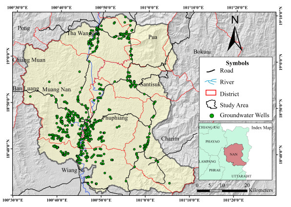
Assessing the capacity of groundwater is essential for efficient water management. Regrettably, evaluating the potential of groundwater in regions with limited data accessibility, particularly in mountainous regions, presents significant challenges. In the Nan basin of Thailand, where there is a scarcity of groundwater well data, we utilized remote sensing and geographic information system (GIS) techniques for evaluating and determining the potential of groundwater resources. The analysis included seven hydrological factors, including elevation, drainage density, lineament density, land use and land cover, slope, soil moisture, and geology. The quantification of groundwater potential was conducted by the utilization of linear combination overlays, employing weights derived from two distinct methodologies: the analytical hierarchy process (AHP) and the frequency ratio (FR). Interestingly, it is noteworthy that both the FR and AHP approaches demonstrated a very comparable range of accuracy levels (0.89–1.00) when subjected to cross-validation using field data pertaining to groundwater levels. Although the FR technique has shown efficacy in situations when data is well-distributed, it displayed constraints in regions with less data, which could potentially result in misinterpretations. On the other hand, the AHP provided a more accurate assessment of the potential of groundwater by taking into account the relative importance of the criteria throughout the full geographical scope of the study. Moreover, the AHP has demonstrated its significance in the prioritization of parameters within the context of water resource management. This research contributes to the development of sustainable strategies for managing groundwater resources.
Citation: Nudthawud Homtong, Wisaroot Pringproh, Kankanon Sakmongkoljit, Sattha Srikarom, Rungtiwa Yapun, Ben Wongsaijai. Remote sensing-based groundwater potential evaluation in a fractured-bedrock mountainous area[J]. AIMS Geosciences, 2024, 10(2): 242-262. doi: 10.3934/geosci.2024014
Assessing the capacity of groundwater is essential for efficient water management. Regrettably, evaluating the potential of groundwater in regions with limited data accessibility, particularly in mountainous regions, presents significant challenges. In the Nan basin of Thailand, where there is a scarcity of groundwater well data, we utilized remote sensing and geographic information system (GIS) techniques for evaluating and determining the potential of groundwater resources. The analysis included seven hydrological factors, including elevation, drainage density, lineament density, land use and land cover, slope, soil moisture, and geology. The quantification of groundwater potential was conducted by the utilization of linear combination overlays, employing weights derived from two distinct methodologies: the analytical hierarchy process (AHP) and the frequency ratio (FR). Interestingly, it is noteworthy that both the FR and AHP approaches demonstrated a very comparable range of accuracy levels (0.89–1.00) when subjected to cross-validation using field data pertaining to groundwater levels. Although the FR technique has shown efficacy in situations when data is well-distributed, it displayed constraints in regions with less data, which could potentially result in misinterpretations. On the other hand, the AHP provided a more accurate assessment of the potential of groundwater by taking into account the relative importance of the criteria throughout the full geographical scope of the study. Moreover, the AHP has demonstrated its significance in the prioritization of parameters within the context of water resource management. This research contributes to the development of sustainable strategies for managing groundwater resources.

| [1] |
Chenini I, Mammou AB (2010) Groundwater recharge study in arid region: An approach using GIS techniques and numerical modeling. Comput Geosci 36: 801–817. https://doi.org/10.1016/j.cageo.2009.06.014 doi: 10.1016/j.cageo.2009.06.014

|
| [2] |
Parisi A, Monno V, Fidelibus MD (2018) Cascading vulnerability scenarios in the management of groundwater depletion and salinization in semi-arid areas. Int J Disaster Risk Reduct 30: 292–305. https://doi.org/10.1016/j.ijdrr.2018.03.004 doi: 10.1016/j.ijdrr.2018.03.004
|
| [3] | Pavelic P, Karthikeyan B, Giriraj A, et al. (2015) Controlling floods and droughts through underground storage: from concept to pilot implementation in the Ganges River Basin, International Water Management Institute (IWMI). |
| [4] |
Choubin B, Malekian A (2017) Combined gamma and M-test-based ANN and ARIMA models for groundwater fluctuation forecasting in semiarid regions. Environ Earth Sci 76: 538. https://doi.org/10.1007/s12665-017-6870-8 doi: 10.1007/s12665-017-6870-8
|
| [5] |
Gopinath G, Seralathan P (2004) Identification of groundwater prospective zones using irs-id liss iii and pump test methods. J Indian Soc Remote Sens 32: 329–342. https://doi.org/10.1007/BF03030858 doi: 10.1007/BF03030858
|
| [6] |
Velis M, Conti KI, Biermann F (2017) Groundwater and human development: synergies and trade-offs within the context of the sustainable development goals. Sustain Sci 12: 1007–1017. https://doi.org/10.1007/s11625-017-0490-9 doi: 10.1007/s11625-017-0490-9
|
| [7] |
Okello C, Tomasello B, Greggio N, et al. (2015) Impact of Population Growth and Climate Change on the Freshwater Resources of Lamu Island, Kenya. Water 7: 1264–1290. https://doi.org/10.3390/w7031264 doi: 10.3390/w7031264
|
| [8] |
Ni B, Wang D, Deng Z, et al. (2018) Review on the Groundwater Potential Evaluation Based on Remote Sensing Technology. IOP Conf Ser Mater Sci Eng 394: 052038. https://doi.org/10.1088/1757-899X/394/5/052038 doi: 10.1088/1757-899X/394/5/052038
|
| [9] | Rao NS, Gugulothu S, Das R (2022) Deciphering artificial groundwater recharge suitability zones in the agricultural area of a river basin in Andhra Pradesh, India using geospatial techniques and analytical hierarchical process method. |
| [10] |
Pathak D, Maharjan R, Maharjan N, et al. (2021) Evaluation of parameter sensitivity for groundwater potential mapping in the mountainous region of Nepal Himalaya. Groundwater Sustainable Dev 13: 100562. https://doi.org/10.1016/j.gsd.2021.100562 doi: 10.1016/j.gsd.2021.100562
|
| [11] |
Amfo-Otu R, Agyenim J, Nimba-Bumah G (2014) Correlation Analysis of Groundwater Colouration from Mountainous Areas, Ghana. Environ Res Eng Manage 1: 16–24. https://doi.org/10.5755/j01.erem.67.1.4545 doi: 10.5755/j01.erem.67.1.4545
|
| [12] |
Voeckler H, Allen DM (2012) Estimating regional-scale fractured bedrock hydraulic conductivity using discrete fracture network (DFN) modeling, Hydrogeol J 20: 1081–1100. https://doi.org/10.1007/s10040-012-0858-y doi: 10.1007/s10040-012-0858-y
|
| [13] |
Smerdon BD, Allen DM, Grasby SE, et al. (2009) An approach for predicting groundwater recharge in mountainous watersheds. J Hydrol 365: 156–172. https://doi.org/10.1016/j.jhydrol.2008.11.023 doi: 10.1016/j.jhydrol.2008.11.023
|
| [14] |
Elewa H, Qaddah A (2011) Groundwater potentiality mapping in the Sinai Peninsula, Egypt, using remote sensing and GIS-watershed-based modeling. Hydrogeol J 19: 613–628. https://doi.org/10.1007/s10040-011-0703-8 doi: 10.1007/s10040-011-0703-8
|
| [15] |
Elmahdy S (2012) Hydromorphological Mapping and Analysis for Characterizing Darfur Paleolake, NW Sudan Using Remote Sensing and GIS. Int J Geosci 3: 25–36. https://doi.org/10.4236/ijg.2012.31004 doi: 10.4236/ijg.2012.31004
|
| [16] |
Jagannathan K, Kumar NV, Jayaraman V, et al. (1996) An approach to demarcate Ground water potential zones through Remote Sensing and Geographic Information System. Int J Remote Sens 17: 1867–1884. https://doi.org/10.1080/01431169608948744 doi: 10.1080/01431169608948744
|
| [17] | Pande CB (2020) Sustainable Watershed Development Planning. In: Sustainable Watershed Development. SpringerBriefs in Water Science and Technology. Springer, Cham. https://doi.org/10.1007/978-3-030-47244-3 |
| [18] |
Pande CB, Moharir KN, Singh SK, et al. (2022) Groundwater flow modeling in the basaltic hard rock area of Maharashtra, India. Appl Water Sci 12: 12. https://doi.org/10.1007/s13201-021-01525-y doi: 10.1007/s13201-021-01525-y
|
| [19] |
Saraf A, Choudhury P, Roy B, et al. (2004) GIS based surface hydrological modelling in identification of groundwater recharge zones, Int J Remote Sens 25: 5759–5770. https://doi.org/10.1080/0143116042000274096 doi: 10.1080/0143116042000274096
|
| [20] |
Swetha TV, Gopinath G, Thrivikramji KP (2017) Geospatial and MCDM tool mix for identification of potential groundwater prospects in a tropical river basin, Kerala. Environ Earth Sci 76: 428. https://doi.org/10.1007/s12665-017-6749-8 doi: 10.1007/s12665-017-6749-8
|
| [21] |
Bhadran A, Girishbai D, Jesiya NP, et al. (2022) A GIS based Fuzzy-AHP for delineating groundwater potential zones in tropical river basin, southern part of India. Geosyst Geoenviron 1: 100093. https://doi.org/10.1016/j.geogeo.2022.100093 doi: 10.1016/j.geogeo.2022.100093
|
| [22] |
Magesh NS, Chandrasekar N (2012) Soundranayagam, J.P. Delineation of groundwater potential zones in Theni district, Tamil Nadu, using remote sensing, GIS and MIF techniques. Geosci Front 3: 189–196, https://doi.org/10.1016/j.gsf.2011.10.007 doi: 10.1016/j.gsf.2011.10.007
|
| [23] |
Zghibi A, Mirchi A, Msaddek MH, et al. (2020) Using Analytical Hierarchy Process and Multi-Influencing Factors to Map Groundwater Recharge Zones in a Semi-Arid Mediterranean Coastal Aquifer. Water 12: 2525. https://doi.org/10.3390/w12092525 doi: 10.3390/w12092525
|
| [24] |
Çelik R (2019) Evaluation of Groundwater Potential by GIS-Based Multicriteria Decision Making as a Spatial Prediction Tool: Case Study in the Tigris River Batman-Hasankeyf Sub-Basin, Turkey. Water 11: 2630. https://doi.org/10.3390/w11122630 doi: 10.3390/w11122630
|
| [25] |
Aghlmand R, Abbasi A (2019) Application of MODFLOW with Boundary Conditions Analyses Based on Limited Available Observations: A Case Study of Birjand Plain in East Iran. Water 11: 1904. https://doi.org/10.3390/w11091904 doi: 10.3390/w11091904
|
| [26] |
Saiz-Rodríguez JA, Lomeli Banda MA, Salazar-Briones C, et al. (2019) Allocation of Groundwater Recharge Zones in a Rural and Semi-Arid Region for Sustainable Water Management: Case Study in Guadalupe Valley, Mexico. Water 11: 1586. https://doi.org/10.3390/w11081586 doi: 10.3390/w11081586
|
| [27] |
Amare S, Langendoen E, Keesstra S, et al. (2021) Susceptibility to Gully Erosion: Applying Random Forest (RF) and Frequency Ratio (FR) Approaches to a Small Catchment in Ethiopia. Water 13: 216. https://doi.org/10.3390/w13020216 doi: 10.3390/w13020216
|
| [28] |
Oh HJ, Kim YS, Choi JK, et al. (2011) GIS mapping of regional probabilistic groundwater potential in the area of Pohang City, Korea. J Hydrol 399: 158–172. https://doi.org/10.1016/j.jhydrol.2010.12.027 doi: 10.1016/j.jhydrol.2010.12.027
|
| [29] |
Saaty TL (1990) How to make a decision: The analytic hierarchy process. Eur J Oper Res 48: 9–26. https://doi.org/10.1016/0377-2217(90)90057-I doi: 10.1016/0377-2217(90)90057-I
|
| [30] |
Pande CB, Moharir KN, Panneerselvam B, et al. (2021) Delineation of groundwater potential zones for sustainable development and planning using analytical hierarchy process (AHP), and MIF techniques. Appl Water Sci 11: 186. https://doi.org/10.1007/s13201-021-01522-1 doi: 10.1007/s13201-021-01522-1
|
| [31] | Mirnazari J, Ahmad B, Mojaradi B., et al. (2014) Using Frequency Ratio Method for Spatial Landslide Prediction. Res J Appl Sci Eng Technol 7: 3174–3180. |
| [32] | Trabelsi F, Lee S, Slaheddine K, et al. (2019) Frequency Ratio Model for Mapping Groundwater Potential Zones Using GIS and Remote Sensing; Medjerda Watershed Tunisia. In: Chaminé H, Barbieri M, Kisi O, et al. (eds), Advances in Sustainable and Environmental Hydrology, Hydrogeology, Hydrochemistry and Water Resources. CAJG 2018. Advances in Science, Technology & Innovation. Springer, Cham, 341–345. https://doi.org/10.1007/978-3-030-01572-5_80 |
| [33] |
Tiwari A, Shoab M, Dixit A (2021) GIS-based forest fire susceptibility modeling in Pauri Garhwal, India: a comparative assessment of frequency ratio, analytic hierarchy process and fuzzy modeling techniques. Nat Hazards 105: 1189–1230. https://doi.org/10.1007/s11069-020-04351-8 doi: 10.1007/s11069-020-04351-8
|
| [34] |
Allafta H, Opp C, Patra S (2020) Identification of Groundwater Potential Zones Using Remote Sensing and GIS Techniques: A Case Study of the Shatt Al-Arab Basin. Remote Sens 13: 112. https://doi.org/10.3390/rs13010112 doi: 10.3390/rs13010112
|
| [35] |
Wood S, Charusiri P, Fenton C (2003) Recent paleoseismic investigations in Northern and Western Thailand. Ann Geophys 46. https://doi.org/10.4401/ag-3464 doi: 10.4401/ag-3464
|
| [36] | DGR (2001) Groundwater Map of Nan Province. |
| [37] |
Rao NS (2009) A numerical scheme for groundwater development in a watershed basin of basement terrain: a case study from India. Hydrogeol J 17: 379–396. https://doi.org/10.1007/s10040-008-0402-2 doi: 10.1007/s10040-008-0402-2
|
| [38] | Rao NS (2012) Indicators for occurrence of groundwater in the rocks of Eastern Ghats. Curr Sci 103: 352–353. https://www.jstor.org/stable/24085075 |
| [39] |
Saaty T (2008) Decision making with the Analytic Hierarchy Process. Int J Serv Sci 1: 83–98. https://doi.org/10.1504/IJSSCI.2008.017590 doi: 10.1504/IJSSCI.2008.017590
|
| [40] | Yahaya S, Ahmad N, Abdalla R (2010) Multicriteria analysis for flood vulnerable areas in Hadejia-Jama'are River basin, Nigeria. Eur J Sci Res 42: 1450–1216. |
| [41] |
Maheswaran G, Selvarani AG, Elangovan K (2016) Groundwater resource exploration in salem district, Tamil nadu using GIS and remote sensing. J Earth Syst Sci 125: 311–328. https://doi.org/10.1007/s12040-016-0659-0 doi: 10.1007/s12040-016-0659-0
|
| [42] | Saaty T, Vargas L (2006) The Analytic Network Process, Decision Making with the Analytic Network Process, 195: 1–26. |
| [43] | Saaty TL (1980) The Analytic Hierarchy Process; McGraw-Hill: New York. |
| [44] |
Manap MA, Nampak H, Pradhan B, et al. (2014) Application of probabilistic-based frequency ratio model in groundwater potential mapping using remote sensing data and GIS. Arab J Geosci 7: 711–724. https://doi.org/10.1007/s12517-012-0795-z doi: 10.1007/s12517-012-0795-z
|
| [45] |
Razavi-Termeh SV, Sadeghi-Niaraki A, Choi SM (2019) Groundwater Potential Mapping Using an Integrated Ensemble of Three Bivariate Statistical Models with Random Forest and Logistic Model Tree Models. Water 11: 1596. https://doi.org/10.3390/w11081596 doi: 10.3390/w11081596
|
| [46] | Koyejo O, Natarajan N, Ravikumar P (2014) Consistent binary classification with generalized performance metrics. Adv Neural Inf Process Syst 3: 2744–2752. |
| [47] | Bekkar M, Djema H, Alitouche TA (2013) Evaluation measures for models assessment over imbalanced data sets. J Inf Eng Appl 3: 27–38. |
| [48] |
Saranya T, Saravanan S (2020) Groundwater potential zone mapping using analytical hierarchy process (AHP) and GIS for Kancheepuram District, Tamilnadu, India. Model Earth Syst Environ 6: 1105–1122. https://doi.org/10.1007/s40808-020-00744-7 doi: 10.1007/s40808-020-00744-7
|
| [49] |
Mohammadi-Behzad HR, Charchi A, Kalantari N, et al. (2019) Delineation of groundwater potential zones using remote sensing (RS), geographical information system (GIS) and analytic hierarchy process (AHP) techniques: a case study in the Leylia–Keynow watershed, southwest of Iran. Carbonates Evaporites 34: 1307–1319. https://doi.org/10.1007/s13146-018-0420-7 doi: 10.1007/s13146-018-0420-7
|
| [50] |
Yeh HF, Cheng YS, Lin HI, et al. (2016) Mapping groundwater recharge potential zone using a GIS approach in Hualian River, Taiwan. Sustainable Environ Res 26: 33–43. https://doi.org/10.1016/j.serj.2015.09.005 doi: 10.1016/j.serj.2015.09.005
|
| [51] |
Jahan CS, Rahaman MF, Arefin R, et al. (2019) Delineation of Groundwater Potential Zones of Atrai-Sib River Basin in North-West Bangladesh using Remote Sensing and GIS Techniques. Sustain Water Resour Manag 5: 689–702. https://doi.org/10.1007/s40899-018-0240-x doi: 10.1007/s40899-018-0240-x
|
| [52] |
Biswas S, Mukhopadhyay BP, Bera A (2020) Delineating groundwater potential zones of agriculture dominated landscapes using GIS based AHP techniques: a case study from Uttar Dinajpur district, West Bengal. Environ Earth Sci 79: 302. https://doi.org/10.1007/s12665-020-09053-9 doi: 10.1007/s12665-020-09053-9
|
| [53] |
Yıldırım Ü (2021) Identification of Groundwater Potential Zones Using GIS and Multi-Criteria Decision-Making Techniques: A Case Study Upper Coruh River Basin (NE Turkey). ISPRS Int J Geo-Inf 10: 396. https://doi.org/10.3390/ijgi10060396 doi: 10.3390/ijgi10060396
|
| [54] |
Benjmel K, Amraoui F, Boutaleb S, et al. (2020) Mapping of Groundwater Potential Zones in Crystalline Terrain Using Remote Sensing, GIS Techniques, and Multicriteria Data Analysis (Case of the Ighrem Region, Western Anti-Atlas, Morocco). Water 12: 471. https://doi.org/10.3390/w12020471 doi: 10.3390/w12020471
|
| [55] |
Maity DK, Mandal S (2019) Identification of groundwater potential zones of the Kumari river basin, India: an RS & GIS based semi-quantitative approach. Environ Dev Sustain 21: 1013–1034. https://doi.org/10.1007/s10668-017-0072-0 doi: 10.1007/s10668-017-0072-0
|
| [56] | Aouragh MH, Essahlaoui ALI, Abdelhadi O, et al. (2015) Using Remote Sensing and GIS-Multicriteria decision Analysis for Groundwater Potential Mapping in the Middle Atlas Plateaus, Morocco. Res J Recent Sci 4: 1–9. |
| [57] |
Boughariou E, Allouche N, Brahim FB (2021) Delineation of groundwater potentials of Sfax region, Tunisia, using fuzzy analytical hierarchy process, frequency ratio, and weights of evidence models. Environ Dev Sustain 23: 14749–14774. https://doi.org/10.1007/s10668-021-01270-x doi: 10.1007/s10668-021-01270-x
|
| [58] |
Ahmadi H, Kaya OA, Babadagi E., et al. (2021) GIS-Based Groundwater Potentiality Mapping Using AHP and FR Models in Central Antalya, Turkey. Environ Sci Proc 5: 11. https://doi.org/10.3390/IECG2020-08741 doi: 10.3390/IECG2020-08741
|
| [59] |
Gautam P, Kubota T, Sapkota LM, et al. (2021) Landslide susceptibility mapping with GIS in high mountain area of Nepal: a comparison of four methods. Environ Earth Sci 80: 359. https://doi.org/10.1007/s12665-021-09650-2 doi: 10.1007/s12665-021-09650-2
|


Figures(5) / Tables(6)

Nudthawud Homtong, Wisaroot Pringproh, Kankanon Sakmongkoljit, Sattha Srikarom, Rungtiwa Yapun, Ben Wongsaijai. Remote sensing-based groundwater potential evaluation in a fractured-bedrock mountainous area[J]. AIMS Geosciences, 2024, 10(2): 242-262. doi: 10.3934/geosci.2024014


 DownLoad: