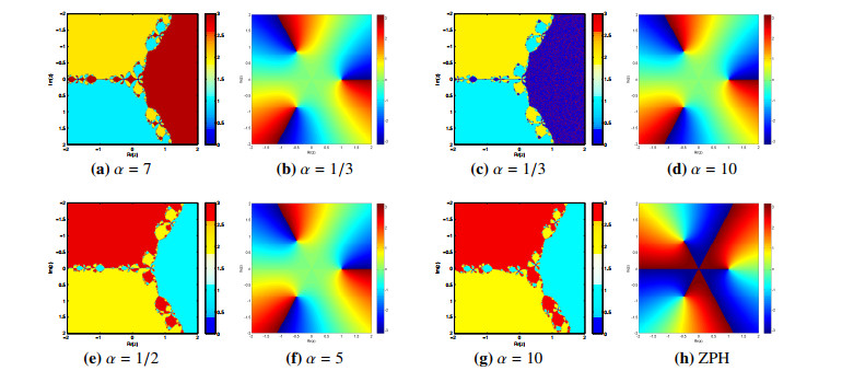
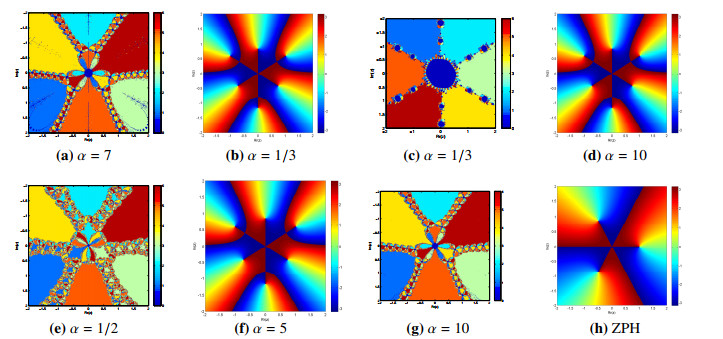
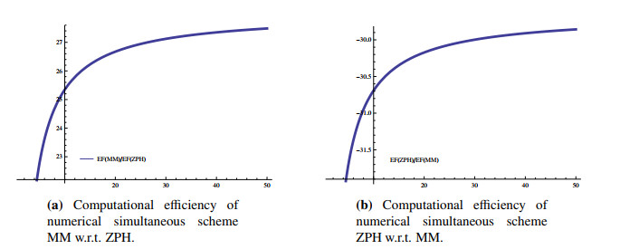
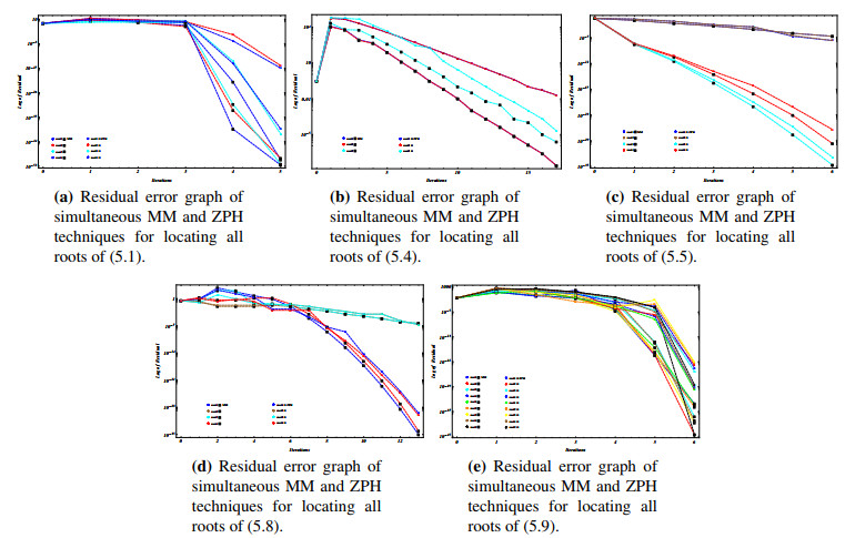
In this article, we constructed a derivative-free family of iterative techniques for extracting simultaneously all the distinct roots of a non-linear polynomial equation. Convergence analysis is discussed to show that the proposed family of iterative method has fifth order convergence. Nonlinear test models including fractional conversion, predator-prey, chemical reactor and beam designing models are included. Also many other interesting results concerning symmetric problems with application of group symmetry are also described. The simultaneous iterative scheme is applied starting with the initial estimates to get the exact roots within the given tolerance. The proposed iterative scheme requires less function evaluations and computation time as compared to existing classical methods. Dynamical planes are exhibited in CAS-MATLAB (R2011B) to show how the simultaneous iterative approach outperforms single roots finding methods that might confine the divergence zone in terms of global convergence. Furthermore, convergence domains, namely basins of attraction that are symmetrical through fractal-like edges, are analyzed using the graphical tool. Numerical results and residual graphs are presented in detail for the simultaneous iterative method. An extensive study has been made for the newly developed simultaneous iterative scheme, which is found to be efficient, robust and authentic in its domain.
Citation: Mudassir Shams, Nasreen Kausar, Serkan Araci, Liang Kong, Bruno Carpentieri. Highly efficient family of two-step simultaneous method for all polynomial roots[J]. AIMS Mathematics, 2024, 9(1): 1755-1771. doi: 10.3934/math.2024085
In this article, we constructed a derivative-free family of iterative techniques for extracting simultaneously all the distinct roots of a non-linear polynomial equation. Convergence analysis is discussed to show that the proposed family of iterative method has fifth order convergence. Nonlinear test models including fractional conversion, predator-prey, chemical reactor and beam designing models are included. Also many other interesting results concerning symmetric problems with application of group symmetry are also described. The simultaneous iterative scheme is applied starting with the initial estimates to get the exact roots within the given tolerance. The proposed iterative scheme requires less function evaluations and computation time as compared to existing classical methods. Dynamical planes are exhibited in CAS-MATLAB (R2011B) to show how the simultaneous iterative approach outperforms single roots finding methods that might confine the divergence zone in terms of global convergence. Furthermore, convergence domains, namely basins of attraction that are symmetrical through fractal-like edges, are analyzed using the graphical tool. Numerical results and residual graphs are presented in detail for the simultaneous iterative method. An extensive study has been made for the newly developed simultaneous iterative scheme, which is found to be efficient, robust and authentic in its domain.

| [1] | S. Akram, M. Junjua, N. Yasmin, F. Zafar, A family of weighted mean based optimal fourth order methods for solving system of nonlinear equations, Life Sci. J., 11 (2014), 21–30. |
| [2] |
A. Cordero, J. García-Maimó, J. R. Torregrosa, M. P. Vassileva, P. Vindel, Chaos in King's iterative family, Appl. Math. Lett., 26 (2013), 842–848. https://doi.org/10.1016/j.aml.2013.03.012 doi: 10.1016/j.aml.2013.03.012

|
| [3] |
P. Agarwal, D. Filali, M. Akram, M. Dilshad, Convergence analysis of a three-step iterative algorithm for generalized set-valued mixed-ordered variational inclusion problem, Symmetry, 13 (2021), 444. https://doi.org/10.3390/sym13030444 doi: 10.3390/sym13030444
|
| [4] |
F. I. Chicharro, A. Cordero, N. Garrido, J. R. Torregrosa, Stability and applicability of iterative methods with memory, J. Math. Chem., 57 (2019), 1282–1300. https://doi.org/10.1007/s10910-018-0952-z doi: 10.1007/s10910-018-0952-z
|
| [5] |
R. Behl, I. K. Argyros, S. S. Motsa, A new highly efficient and optimal family of eighth order methods for solving nonlinear equations, Appl. Math. Comput., 282 (2016), 175–186. https://doi.org/10.1016/j.amc.2016.02.010 doi: 10.1016/j.amc.2016.02.010
|
| [6] |
C. Chun, Y. I. Kim, Several new third-order iterative methods for solving nonlinear equations, Acta Appl. Math., 109 (2010), 1053–1063. https://doi.org/10.1007/s10440-008-9359-3 doi: 10.1007/s10440-008-9359-3
|
| [7] |
F. Zafar, A. Cordero, J. R. Torregrosa, An efficient family of optimal eighth-order multiple root finders, Mathematics, 6 (2018), 310. https://doi.org/10.3390/math6120310 doi: 10.3390/math6120310
|
| [8] | J. M. McNamee, Numerical Methods for Roots of Polynomials, Part II, Amsterdam: Elsevier, 2013. |
| [9] |
G. H. Nedzhibov, Iterative methods for simultaneous computing arbitrary number of multiple zeros of nonlinear equations, J. Comput. Math., 90 (2013), 994–1007. https://doi.org/10.1080/00207160.2012.744000 doi: 10.1080/00207160.2012.744000
|
| [10] | P. D. Proinov, M. T. Vasileva, On the convergence of family of Weierstrass-type root-finding methods, C. R. Acad. Bulg. Sci., 68 (2015), 697–704. |
| [11] |
N. A. Mir, R. Muneer, I. Jabeen, Some families of two-step simultaneous methods for determining zeros of non-linear equations, ISRN Appl. Math., 2011 (2011), 817174. https://doi.org/10.5402/2011/817174 doi: 10.5402/2011/817174
|
| [12] | S. I. Cholakov, Local convergence of Chebyshev-like method for simultaneous finding polynomial zeros, C. R. Acad. Bulg. Sci., 66 (2013), 1081–1090. |
| [13] |
P. D. Proinov, M. T. Vasileva, On a family of Weierstrass-type root-finding methods with accelerated convergence, Appl. Math. Comput., 273 (2016), 957–968. https://doi.org/10.1016/j.amc.2015.10.048 doi: 10.1016/j.amc.2015.10.048
|
| [14] |
P. D. Proinov, M. D. Petkova, A new semilocal convergence theorem for the Weierstrass method for finding zeros of a polynomial simultaneously, J. Complexity, 30 (2014), 366–380. https://doi.org/10.1016/j.jco.2013.11.002 doi: 10.1016/j.jco.2013.11.002
|
| [15] |
M. G-S´anchez, M. Noguera, A. Grau, J. R. Herrero, On new computational local orders of convergence, Appl. Math. Lett., 25 (2012), 2023–2030. https://doi.org/10.1016/j.aml.2012.04.012 doi: 10.1016/j.aml.2012.04.012
|
| [16] |
S. I. Ivanov, A unified semilocal convergence analysis of a family of iterative algorithms for computing all zeros of a polynomial simultaneously, Numer. Algor., 75 (2017), 1193–1204. https://doi.org/10.1007/s11075-016-0237-1 doi: 10.1007/s11075-016-0237-1
|
| [17] |
S. Kanno, N. V. Kjurkchiev, T. Yamamoto, On some methods for the simultaneous determination of polynomial zeros, Japan J. Indust. Appl. Math., 13 (1995), 267–288. https://doi.org/10.1007/BF03167248 doi: 10.1007/BF03167248
|
| [18] | K. Weierstrass, Neuer beweis des Satzes, dass jede ganze rationale function einer veränderlichen dargestellt werden kann als ein product aus linearen functionen derselben veränderlichen, Ges. Werke, 1981, 1085–1101. |
| [19] | I. O. Kerner, Ein gesamtschrittverfahren zur berechnung der nullstellen von polynomen, Numer. Math., 8 (1966), 290–294. |
| [20] | E. Durand, Solutions numeriques des equations algebriques, tome 1: Equations du Type $F(\varkappa) = 0$, Racines dun Polynome, Masson, 17 (1960), 540–546. |
| [21] | K. Dochev, Modified Newton methodfor the simultaneous computation of all roots of a given algebraic equation, in Bulgarian, Phys. Math. J. Bulg. Acad. Sci., 5 (1962), 136–139. |
| [22] | S. B. Presic, Un proced e iteratif pour la factorisation des polynomes, C. R. Acad. Sci. Paris. Ser. A., 262 (1966), 862–863. |
| [23] |
P. D. Proinov, General convergence theorems for iterative processes and applications to the Weierstrass root-finding method, J. Complexity, 33 (2015), 118–144. https://doi.org/10.1016/j.jco.2015.10.001 doi: 10.1016/j.jco.2015.10.001
|
| [24] | G. H. Nedzhibov, Improved local convergence analysis of the Inverse Weierstrass method for simultaneous approximation of polynomial zeros, In: Proceedings of the MATTEX 2018 Conference, Targovishte, Bulgaria, 1 (2018), 66–73. |
| [25] |
P. I. Marcheva, S. I. Ivanov, Convergence analysis of a modified Weierstrass method for the simultaneous determination of polynomial zeros, Symmetry, 12 (2018), 1408. https://doi.org/10.3390/sym12091408 doi: 10.3390/sym12091408
|
| [26] | J. S. Song, Simultaneous methods for finding all zeros of a polynomial, J. Math. Sci. Adv. Appl., 33 (2015), 5–18. |
| [27] |
H. Ren, Q. Wu, W. Bi, A class of two-step Steffensen type methods with fourth-order convergence, Appl. Math. Comput., 209 (2009), 206–210. https://doi.org/10.1016/j.amc.2008.12.039 doi: 10.1016/j.amc.2008.12.039
|
| [28] |
X. Zhang, H. Peng, G. Hu, A high order iteration formula for the simultaneous inclusion of polynomial zeros, Appl. Math. Comput., 179 (2006), 545–552. https://doi.org/10.1016/j.amc.2005.11.117 doi: 10.1016/j.amc.2005.11.117
|
| [29] |
M. Shams, N, Rafiq, N. Kausar, P. Agarwal, C. Park, N. A. Mir, On highly efficient derivative-free family of numerical methods for solving polynomial equation simultaneously, Adv. Differ. Equ., 2021 (2021), 465. https://doi.org/10.1186/s13662-021-03616-1 doi: 10.1186/s13662-021-03616-1
|
| [30] |
I. K. Argyros, Á. A. Magreñán, L. Orcos, Local convergence and a chemical application of derivative free root finding methods with one parameter based on interpolation, J. Math. Chem., 54 (2016), 1404–1416. https://doi.org/10.1007/s10910-016-0605-z doi: 10.1007/s10910-016-0605-z
|
| [31] | L. Edelstein-Keshet, Differential Calculus for the Life Sciences, Vancouver: Univeristy of British Columbia, 2017. |
| [32] | J. L. Zachary, Introduction to Scientific Programming: Computational Problem Solving Using Maple and C, New York: Springer, 2012. |
| [33] | A. Constantinides, M. Mostoufi, Numerical Methods for Chemical Engineers with MATLAB Applications, New Jersey: Prentice Hall PTR, 1999. |
| [34] | J. M. Douglas, Process Dynamics and Control, Englewood Cliffs: Prentice Hall, 1972. |
| [35] | M. R. Farmer, Computing the zeros of polynomials using the Divide and Conquer approach, Ph.D thesis, Department of Computer Science and Information Systems, Birkbeck, University of London, 2014. |
| [36] |
M. S. Petkovic, L. D. Petkovic, Construction of zero-finding methods by Weierstrass functions, Appl. Math. Comput., 184 (2007), 351–359. https://doi.org/10.1016/j.amc.2006.05.159 doi: 10.1016/j.amc.2006.05.159
|
Figures(4) / Tables(13)

Mudassir Shams, Nasreen Kausar, Serkan Araci, Liang Kong, Bruno Carpentieri. Highly efficient family of two-step simultaneous method for all polynomial roots[J]. AIMS Mathematics, 2024, 9(1): 1755-1771. doi: 10.3934/math.2024085


 DownLoad: